Revisit Basic Math of Machine Learning
Matrix-Vector Revisit
Matrix and Vector Norm
Vector Norm
- measure the size of a vector (measure the distance from the origin to the point )
- When , we have the Euclidean form
Matrix Norm
- Frobenius norm measures the size of a matrix
- If A is symmetric, Frobenius norm measures the sum of the variation along all dimension.
Multiplying Matrix and Vector
Dot product of two vector
Matrix-vector multiplication
Matrix-matrix multiplication
- is matrix
- is matrix
- is an matrix
- is an matrix
- is the batch size or the number of input vectors

Vector Space
- A vector space is a set of objects called vectors, which may be added together and multiplied (“scaled”) by numbers, called scalars.
Example, a vector on a 3-D vector space [X=2, Y=3, Z=5]

Subspace
- In linear algebra, a linear subspace is a vector space that is a subset of some larger vector space.

- Linear = Subspace
- Non-linear = Manifold
Is the curve surface (2-D manifold) a linear subspace of a 3-dimensional space?
- No. It is non-linear subspace.
Revisit Random Variables and Probability Distributions
Random Variables (RV)
-
A Random Variable is a variable whose value is subject to variation due to chance
-
Random Variable can be discrete:
- E.g. an Random Variable could be X = no. of heads after flipping a fair coin 2 times, Then X can only be 0 or 1 or 2.
- E.g Throw a fair dice once
- Discrete Probability Distribution is also called Probability Mass Function (PMF)
-
Random Variable can also be continuous:
- E.g. Weight of a person; can take on any value within an interval
-
 * The Majority weight is 200 in this case. (Most likely 200 from the view of probability)
-
- Continuous Probability Distribution is also called Probability Density Function (PDF)
- E.g. Weight of a person; can take on any value within an interval
-
The function describing the possible values of an Random Variable and their associated probabilities is known as a probability distribution.

Histogram and Probability Density Function (PDF)
- For a continuous random variable, the histogram converges to PDF when the bin size goes to zero

Conditional Probability

- : Joint Probability Density Function of and
- and : The Two conditional probability distributions
- These are formed by extracting the appropriate slice from the joint pdf and normalizing so that the area is one. A similar operation can be performed for discrete distributions
Rules of Probability
joint probability
: marginal probability
conditional probability
Sum Rule
Discrete case : Summation
Continuous case : Integration
If Y is Continuous,
Product Rule
Discrete RV in Machine Learning
-
In machine learning, discrete probability distributions are often used for modeling binary and multi-class classification problems
-
E.g. Gender Classification from their facial image x (Binary classification problem)
- and Female
- is a random variable with possible outcomes “Male” or “Female”.
- follows a Bernoulli distribution.
-
E.g. Classification of handwritten digit with image x (Multi-class classification problem)
- , where and
- is a random variable with possible outcomes {0,1,⋯,9}
- follows a Multinoulli (categorical) distribution.
Continuous RV in Machine Learning
-
In machine learning, continuous probability distributions are often used for modeling feature vectors
-
E.g. Assume that facial image x follows a Gaussian distribution
-
-
x is a random vector (variable) with infinite number of possible outcomes
-

- mean have the highest chance of occuring
- Note , just like any PDF.
-
Expectation for Discrete RV
For discrete RV, the expectation (expected value) of a function with respect to a probability distribution is average value that f takes on when is drawn from :
- Upper case Is used to denote discrete probability distribution
-
If P is uniform, Expected value = mean
-
If P is not uniform, Expected valued = weighted mean
-
E.g. Throw a fair dice
-
-
Expectation for Continuous RV
For continuous RV, the expectation (expected value) of a function with respect to a probability distribution is the average value that f takes on when is drawn from :
- Lower case is used to denote continuous probability distribution
- Expectation of samples drawn from a Gaussian distribution

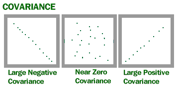
Variance and Covariance
Variance gives a measure of how much the values of a function f of a random variable vary as we draw samples from the probability distribution of :
Variance of f(x) = Expectation[ ( f(x) - Expectation[f(x)] )^2 ]
Note Expectation[f(x)] = mean
The covariance measures how much two functions of RVs (x and y) are linearly related to each other, as well as the scale of these variables:
Covariance of f(x) and g(y) = Expectation[ ( f(x) - Expectation[f(x)] ) ( g(y) - Expectation[g(y)] ) ]
- Positive covariance means when x is large (small), y is also large (small)
- Negative covariance means when x is large (small), y is small (large)
covariance In vector form:
- Note now is a matrix
Note the symmetric properties in Covariance Matrix.
E.g.
For
For
Note
Variance and Covariance Relation to Machine Learning
- Many machine learning problems are multivariate, e.g., an image with 28 x 28 pixels can be viewed as a 784-dim vector
- Neighboring pixels are positive correlated for smooth images.
- We use a covariance matrix to quantify the variances and the covariances of different pixels:

Bayes Theorem and Its Role in Classification Systems
Bayes theorem states the following:
- Prior: Probability distribution representing knowledge or uncertainty of a data object prior or before observing it
- Posterior: Conditional probability distribution representing what parameters are likely after observing the data object
- Likelihood: The probability of falling under a specific category or class.
Bayes Theorem

E.g.
Assume is our measurement (weight),
Prior =
Likelihood =
Posterior = Likelihood * Prior
If Y is discrete:
e.g., X is the height of a person and Y is his/her gender (‘M’ or ‘F’)
If Y is continuous:
e.g., X is the weight of a person and Y his/her wealth
Note: When is continuous, likelihood is not probability and could be greater than 1
E.g. When x is too small e.g. 0.0001, p(X|Y) need to be higher than 1 to compansate that the PDF area is equal to 1.
Only in continuous, likelihood is different from probability
If x is a continuous random variable, the likelihood of x could be larger than 1.
- Yes
Example:
Bayes Theorem:
Therefore:
Marginal Density =

Bayes Decision Theory
Decision Rule for 2-class problems: ( means class1, means class2)
- Where is Prior.

Decision Rule for K-class problems: ( means class k)
- Where is Prior.

Gaussian Mixture Model
- Sometime the distribution may not be Gaussian.
- A Gaussian mixture model is a linear combination of M Gaussian densities:

^ is weight, is the number of gaussian distributions

http://ethen8181.github.io/machine-learning/clustering/GMM/GMM.html
In GMM, each cluster corresponds to a probability distribution, in this case the Gaussian distribution. What we want to do is to learn the parameters of these distributions, which is the Gaussian’s mean , and the variance .
Note The mathematical form of the Gaussian distribution in 1-dimension (univariate Gaussian) can be written as:
- This is also referred to as the probability density function (pdf).
- Gaussian distribution is commonly referred to as the Normal distribution, hence that’s where the comes from.
- refers to the random observation over which this distribution is placed.
- The mean , controls the Gaussian’s “center position” and the variance , controls its “shape”. To be precise, it is actually the standard deviation , i.e. the square root of the variance that controls the distribution’s shape.
In higher dimensions, a Gaussian is fully specified by a mean vector and a d-by-d covariance matrix, (do not confused this symbol with , which is used for denoting summing a bunch of stuff). refers to the determinant of the covariance matrix e.g. In two dimension, the Gaussian’s parameters might look like this:
The mean vector, containing elements and centers the distribution along every dimension. On the other hand, the covariance matrix specifies the spread and orientation of the distribution. Along the diagonal of this covariance matrix we have the variance terms and representing the shape (spread) along each of the dimensions. But then we also have the off-diagonal terms, and (these two thing actually take the same value because this a symmetric matrix) that specify the correlation structure of the distribution.
Remember the covariance matrix is symmetric.
- Diagonal covariance matrix (off-diagonal terms are zero)
- Full covariance matrix (off-diagonal terms are non-zero)
Gaussian Mixture Model Classifier (GMM Classifier)
Given a data set comprising the samples of K classes, we partition the data into K class-dependent subsets:
We use the samples in Class to train the -th GMM:
During classification, given an unknown vector x, we use the Bayes theorem to decide its class label :
Note the training of individual GMMs is unsupervised,
but the construction of the GMM classifier is supervised.
- The training of a GMM is unsupervised in that only the feature vectors are used for training the k-th GMM.
- We also did not train the GMM to map x to a class label c.
- Instead, we train the k-th GMM to generate the data in the k-th class.
- To use GMMs for classification, we train one GMM per class. So, the label information of the training data is implicitly used when constructing a GMM classifier.
Support Vector Machines
- During the second AI winter, support vector machine (SVM) is an important machine learning model.
- It is very good at performing classification tasks
- Even with the recent advances in deep neural networks, SVM still plays an essential role in many practical systems.
- In many real-word problems, we do not have enough data to train a DNN for the classification tasks.
- Suitable for small amount of data
- One solution is to train a DNN using massive amount of data from another similar data source and use the DNN as feature extractor (called embedding). Then, we use the small number of feature vectors to train an SVM for our task.
Margin Maximization
- SVM is trained by maximizing the margin between the hyperplanes of two classes

- We aim to find a decision plane that maximizes the margin to obtain
SVM Classifier
- SVM is good for binary classification.
- To classify multiple classes, we can use the one-vs-rest approach to convert K binary classifications to a K-class classification

Explain why it is always possible to use a plane (linear SVM) to divide 3 linearly independent samples into two classes. What happens when the 3 samples are linearly dependent?
- When the 3 samples are not linearly dependent, they should span a plane on the 3-D space, i.e., they become the corners of a triangle. As a result, a linear SVM can classify the 3 points perfectly.
- On the other hand, when the 3 points are co-linear (linearly dependent), they form a line on the 3-D space. All points on the line can be specified by the first two dimensions, because the third dimension depends on the first two. As we now have more points (N = 3) than the dimension of feature vectors (D = 2), we need a non-linear classifier such as RBM-SVM. The following diagram illustrates such situation.

The support vectors of an SVM are usually near the decision boundary?
Yes.
MLP vs GMM vs SVM
- You may consider GMM and SVM as a special form of MLP with only one hidden layer, one output, and with a special activation function


Why can we consider Gaussian mixture models (GMMs) and support vector machines with non-linear kernel functions (e.g., RBF-SVM) as neural networks with a single hidden layer?
The forward propagation equations of GMMs and RBF-SVMs are linear weighted sum of some non-linear functions. Therefore, the equations have the same form as a neural network with one hidden layer.
Why can we consider Gaussian mixture models (GMMs) and support vector machines with non-linear kernel functions (e.g., RBF-SVM) as neural networks with a single hidden layer?
- The forward propagation equations of GMMs and RBF-SVMs are linear weighted sum of some non-linear functions. Therefore, the equations have the same form as a neural network with one hidden layer.

Questions

1(a)
For distributions with a common covariance structure the decision regions are hyper-planes.


1(b)
For distribution with arbitrary covariance structures the decision regions are defined by hyper-spheres.


2(a)
As none of the central pixels (14, 14) in the 5,000 training samples contains the strokes of Digit ‘0’, that means there is no 0.6~1 intensity. As the digits were contaminated by Gaussian noise, there is also no frequency of 0 intensity is also 0. we can assume the histogram is actually a gaussian PDF if bin = 0, and it won’t fall into the range of 0.6 to 1 (Which is the stroke level intensity) and 0 (because of contamination).


2(b)
Recall Formula of GMM Classifier:
Given a data set comprising the samples of K classes, we partition the data into K class-dependent subsets:
We use the samples in Class to train the -th GMM:
During classification, given an unknown vector x, we use the Bayes theorem to decide its class label :
Therefore:
We first convert the training images into vectors by stacking the pixels, which result in 5000 training vectors per digit. Then, we train 10 Gaussian models (density function) with mean vectors and covariance matrices , one for each digit. A Gaussian classifier is formed as follows:

2©
Given a test vector x, the Gaussian classifier determines the class label of x by the following formula:
where is the likelihood of x given the Gaussian model of Digit . The prior probability is obtained as follows:

2(d)
No. This is because 100 samples could not produce a full covariance matrix with valid inverse.
it’ll change the rank of the cov matrix apparently.

2(e)
Change the full covariance matrices to diagonal covariance matrices. Because each element in the diagonal is now estimated by 100 samples, the variance is reliable and will not be 0.
Because diagonal matrix is always inversible as long as no term is zero and variance is always a positive, non zero number. So diagonal matrix is reliable.

2(f)
When the number of training sample per digit is 1, using diagonal covariance matrices will not help because the variances are still 0. In such situation, we may use a common diagonal covariance matrix for all of the 10 digits so that each diagonal element will be estimated by 10 numbers. Then, the variance will not be 0. A better solution is NOT to use Gaussian classifier, e.g., using linear SVM instead.