Summary of iconic Image Segmentation methods
Quick Review of CNN and relvent terms
CNN
- Reduce the sizes of filters (keep only useful features)
- Parameter sharing (How?)
- 2D Filter slide through the weights (Convolution)
- Convolution extract features and represent it with smaller size
- The convolution results show the similarity at various positions (correlation amount data)
- Convolution extract features and represent it with smaller size
- 2D Filter slide through the weights (Convolution)
- Interence function:
- Training:
-
- Hence can be found
Feature map width = (Width - FilterSize + 2 * Padding ) / (Stride) + 1
Padding
- Zero padding: add zero padding
- Valid convolution means no padding
- same convolution means pad the corners so that output size = input size
Pooling (Subsampling)
- Often used after the convolutional layer to reduce spatial size (only width and height, not the depth)
- Max pooling: return maximum value from the portion of the image covered by the kernel
- Average pooling: returns the average value from the portion of the image covered by the kernel.
Filters
- Image is in (Width, Height, Depth) where depth = 3
- We can slide a WxHx3 filter over the image and obtain a activation map which serves as the input to the next layer
- We use multiple filters where each filter produce one frame
Standard CNN arch
- Feature Extraction Stage (CNNs) => Flatten => Fully Connected Layers => Out
LeNet (LeCun, 1998)
- Conv-Pool-Conv-Pool-Flatten-FC-FC-FC-Out
- Used Tanh and Sigmoid => Suffer from gradient vanishing problem
- Why LeNet was not popular at that time?
- Limitation of computational power
- Weak theoretical background: researchers appreciated methods with mathematical proof such as SVM
AlexNet (2012)
-
First to use ReLU
-
Data Augmentation
- Image pre-processing and cropping
- Horizontal reflection
- Color jittering
- step1: Computer PCA on all RGB points valuese in the training image
- step2: Sample somecolor offset along the principal components at each forward pass annd add random variable drawn from a gaussian with
- step3: add the offset to all pixels in a training image
-
Dropout
- Randomly drop out connections between input and output in each weight update cycle.
- Hence, every input goes through a different network architecture.
- Increase difficulty for the network the memorize the training data very well and increase the robustness of the network
- Hence, every input goes through a different network architecture.
- Randomly drop out connections between input and output in each weight update cycle.
-
Large filter size used (filters in 1st layer are 11x11)
- Filter sizes affect number of trainable parameters and large filter size would be too aggressive for training
VGGNet (2014)
- Deeper layers
- Smaller filter (Standardized all filters to 3x3)
- Note the receptive field of two 3x3 conv layers is equal to a 5x5.
- However using 5x5 filter has 5*5+1 =26 params,
- while using two 3x3 filters have 2(3*3+1) = 20 params
- Note the receptive field of two 3x3 conv layers is equal to a 5x5.
GoogleNet (2014)
- Inception module
- Parallel combination of 1x1, 3x3, 5x5 conv filters and make a concatenation (bottleneck layer) to obtain the same size output
Deep Learning for Image Segmentation
- Local segmentation
- FCN
- U-Net
Local segmentation
How Local segmentation is done?
- 1: Extract a patch from an image, then use a classification model to classify
- 2: Re-extract patch from the image in the next pixel, then use a classification model to classify again
- 3: Repeat 1 and 2 until all pixels are searched
- 4: Able to locate the thing
Drawbacks of Local segmentation
- Very slow because network is run separately for each patch
- Patch size determine the localization accuracy (trade-off in the use of context)
- Larger patch => lower localization accuracy, but better use of context
- Smaller patch => higher localization accuracy, but worse use of context
FCN (Fully Convolutional Network)
- Pixelwise prediction: trained end-to-end, pixels-to-pixels
- Both learning and inference are performed whole-image-at-a-time
- Supervised (Need training dataset with labels)
- Outperform local segmentation in terms of efficiency and quality
- Can be applied on images of any resolution
- In FCN, input is , output is also
How FCN works?
- Only uses Convolutional layers to extract image from to
- Convolutional layers contains Conv, Pool and nonlinearity
- If we upsample the output, we can calculate the pixelwise output (label map).
- How to upsample the output?
Upsample an image using Convolution with Fractional Strides
-
Convolution with Fractional Strides is also known as Deconvolution, Up Convolution, Transposed Convolution
-
Insert columns and rows of zero between neighboring columns and rows
- Fractional stride indicates the amount of zero columns and rows to be inserted
- Strides of 1/S: enlarge the image resoltuion by S times
- We can use Strides 1/32 to turn the label map with size into image with dim
- Is this upsampling approach too aggressive?
- We can incorporate information from previous (lower-level) feature layers
- We can use Strides 1/32 to turn the label map with size into image with dim

Drawbacks of FCN
- Needs a lot of training pairs (~10k labeled images)
- Result quality is not satisfactory due to blur boundaries
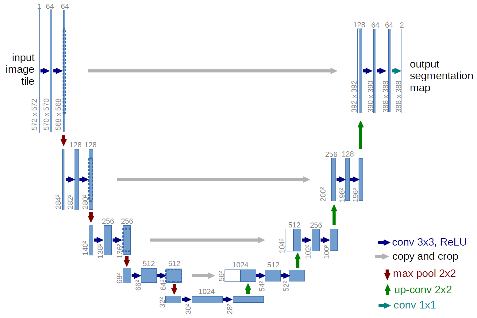
U-Net
-
Built upon FCN with two main differences
-
Many feature channels in the upsampling part
- Allow the network to propagate context information to higher resolution layers. Therefore, the expansive path is more or less symmetric to the contracting path, and yields a u-shaped architecture
- Yield more precise segmentations
-
Excessive data augmentation by applying elastic deformation to the training images
- Allow the network to learn invariance to such deformations without the need to see these transformations in the annotated image corpus
How U-Net works?
-
Encoder-Decoder body
-
Skipping layers and directly transmit the information to the target layer
- Cropping is required before skipping layers due to the loss of border pixels in every convolution
-
To predict the pixels in the border region of the image, the missing context is extrapolated by mirroring the input image.
-
Data augmentation applied to both input and ground-truth images together
- Eg. Random crop, flip, translate, rotate, scale, skew etc
- UNet proposed Elastic Deeformations