Some Practice Questions on DNN

Deep Learning Basics

Are deep learning and deep neural networks the same thing?

No

What is the relationship between deep learning and machine learning?

Deep learning is a kind of machine learning

The weight connecting artificial neurons of a neural network represents the strength of the signal passing between biological neurons. Is it true?

True

Will close-form solution work in gradient-based methods?

If there is a closed form solution for the derivative of the loss function, we can simply find the weights by solving equations, that is called the close-form solution.

However, in practice, the relationship between the loss function and the network weights is very complex. Setting the derivative to zero will not lead to a closed-form solution.

(a)(i)

• Number of Inputs: 28x28 = 784
• Number of outputs: 10

(a)(ii)

The bias terms are to allow the network to produce decision boundaries that lie on any regions of the feature space, not necessarily passing through the origin.

• Activation function: Softmax
  • let the network produce posterior probabilites of individual classes
• Objective function: Cross-entropy
  • the function is differentiable and is closest to the classification error. It also emphasizes the error on the correct class

If all hidden nodes are linear, the multiple layers reduce to a single layer and the advantages of deep architecture is lost. Mathematically, denote $\mathbf{x}$ as the input and $\mathbf{W}_{l}, l=1, \ldots, L$ as the weights (including bias terms) of the hidden layers. When all hidden neurons are linear, then the network outputs become

$$\mathbf{y}=\operatorname{softmax}\left(\mathbf{W}_{L} \mathbf{W}_{L-1} \cdots \mathbf{W}_{1} \mathbf{x}\right)=\operatorname{softmax}(\mathbf{W} \mathbf{x})$$

where $\mathbf{W}=\mathbf{W}_{L} \mathbf{W}_{L-1} \cdots \mathbf{W}_{1}$. This is equivalent to multi-class logistic regression.

Model Capacity (Concept)

When gradient vanishing is not an issue and that the amount of training data is very large, a deep neural network can provide more abstract representation of the features. The degree of abstraction increases from the bottom layers to the upper layers. Very abstract features are close to the classification task, making classification easy. In fact, if the features are abstract enough, a linear layer with a softmax output can readily classify the highly abstract features. For example, in face recognition, a deep network with sufficient layer can represent different types of faces (e.g., large eyes, big nose, big eyebrow, etc.) in the last hidden layer, making the softmax layer to be able to classify the face easily. On the other hand, the hidden layers in a shallow network can only represent some primitive features of the faces (e.g., round edge, sharp edge, round hole, etc.), making classification difficult.

Can deep neural networks be used as feature extractor?

Yes

Model Hidden Layer (Concept)

5a)

As shown in the above figure, the outputs of the hidden nodes are a function of the linear weighted sum of inputs plus a bias. If the sigmoid function f() has a steep sloop, its output over a range of input x1 and x2 will look like the following figure. The left and right figures correspond to the output of hidden neurons 1 and 2, respectively. The first neuron maps data above L1 to 0.0 and below L1 to 1.0. Similarly, the second neuron maps data above L2 to 1.0 and below L2 to 0.0. The resulting mapping are shown in the bottom figure. The output neuron separates the data in the 2-D space defined by the hidden node outputs ($o_1^{(1)}$and $o_2^{(1)}$). As can be seen, the data on this new space are linearly separable and can be easily classified by L3, which is produced by the output neuron.

5b)

Optimization

SGD and Momentum (Concept)

Revisit:

• Gradient Decent

  • Use all samples to calculate derivatives for each step
  • Too expensive when the sample size is big

• Stochastic Gradient Decent

  • Randomly pick one sample to calculate derivatives for each step
  • Save computation (update the parameters with just the new data)
  • Easily to update parameters when new data shows up

• Mini-batch Gradient Decent:

  • Randomly pick a small subset of samples to calculate derivatives for each step
  • Save computation

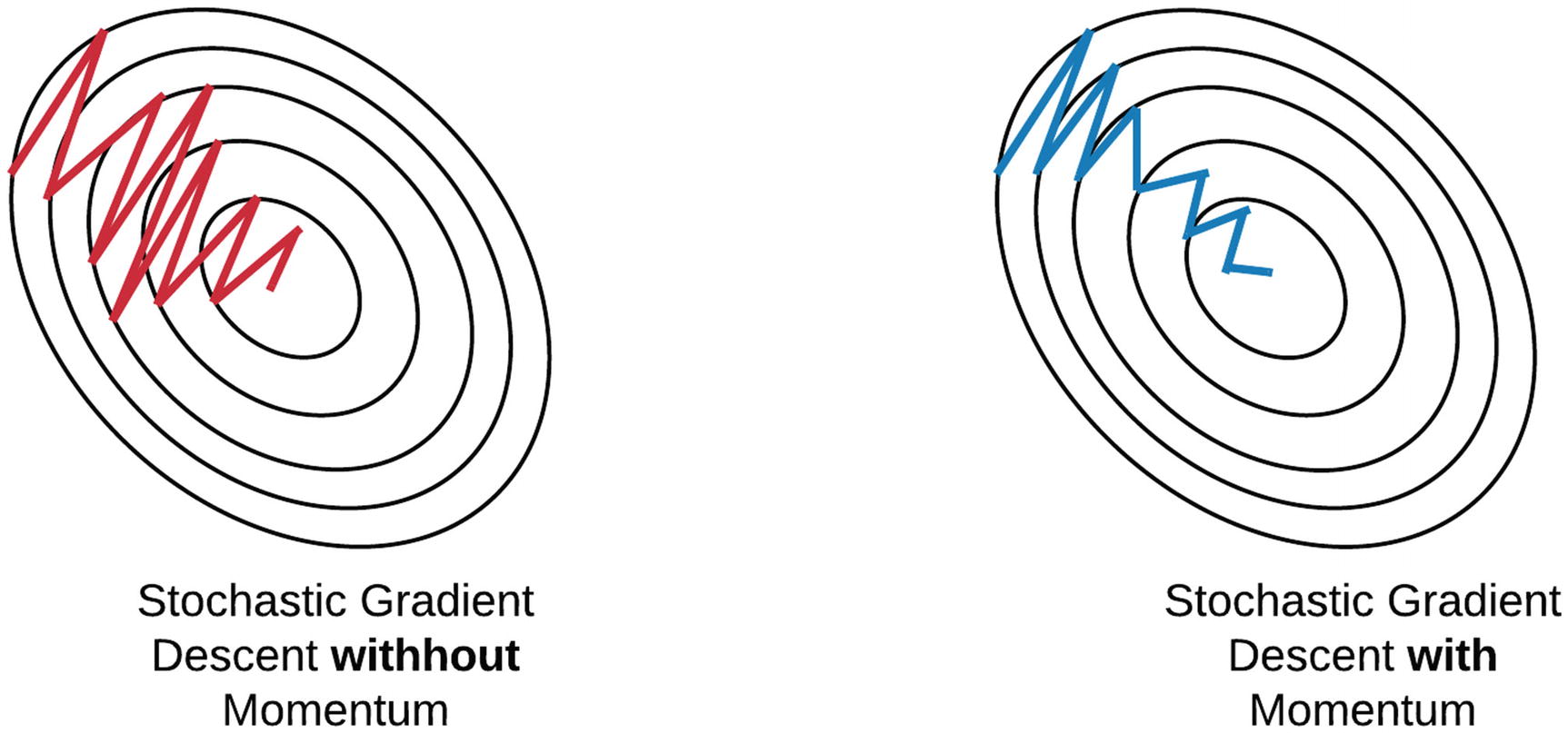
But we can see:

• Stochastic or Mini-Batch Gradient Descent, the points in training steps are oscillating.

• For Gradient Descent, Oscillation problem could also exist when there is a large learning rate.

  

• Oscillation means the point landed on unintended regions of the error surface.

The momentum is designed to minimize the oscillation. With momentum, ends up eventually taking steps with much smaller oscillation.

Formula of Gradient Descent without momentum

the weights at the t-th update (not epoch) are changed according to the gradient with respect to the weights as follow:

$$\begin{array}{c} \Delta \mathbf{w}(t)=\eta \frac{\partial E(t)}{\partial \mathbf{w}} \\ \mathbf{w}(t)=\mathbf{w}(t-1)-\Delta \mathbf{w}(t) \end{array}$$

Formula of Gradient Descent with momentum

the weights at the t-th update (not epoch) are changed according to the gradient with respect to the weights as follow:

$$\begin{array}{c} \Delta \mathbf{w}(t)=\eta \frac{\partial E(t)}{\partial \mathbf{w}}+\gamma \Delta \mathbf{w}(t-1) \\ \mathbf{w}(t)=\mathbf{w}(t-1)-\Delta \mathbf{w}(t) \end{array}$$

With the momentum term $\gamma \Delta \mathbf{w}(t-1), \Delta \mathbf{w}(t)$ is now pointing to a direction between the current gradient and the previous update, as shown in the figure below.

Therefore, the update path will become closer to the ideal path as shown below.

When the error surface is symmetric across all dimensions, the momentum term still plays a role in stochastic gradient descent. Is this true?

True.

When the error surface is symmetric across all dimensions, the gradient update won’t encounter situation like the direction update.

However, it will encounter the situation when it overshoots the minimum point, so the momentum will helps the update and correct the update direction. Therefore, the momentum term still plays a role.

Gradient Decent (Math Derivation)

Loss function Binary Cross-Entropy (Ignored index for simplicity):

$$E=-t \log y-(1-t) \log (1-y)$$

Note the derivative of sigmoid:

If $o = h(a) = \frac{1}{1+e^{-a}}$

then, $\frac{\partial{o}}{\partial{a}}=h'(a) = o(1-o)$

First we define the forward propagation.

Output layer

$$y = h(a_i^{(2)})$$

$$a^{(2)}_i = \sum_iw_{ji}^{(2)}o^{(1)}_j$$

The first hidden layer

$$o^{(1)}_j = h(a_j^{(1)})$$

$$a_j^{(1)}=\sum_iw_{ji}^{(1)}x_i$$

And now we know $E$ depends all the $y$ terms, and $y$ depends all the $a$ terms.

Now we can find the gradients with respect to the weights at the first hidden layer:

$$\frac{\partial E}{\partial w_{i j}^{(2)}}=\frac{\partial E}{\partial a_{i}^{(2)}} \frac{\partial a_{i}^{(2)}}{\partial w_{1 j}^{(2)}}$$

$$\frac{\partial a_{i}^{(2)}}{\partial w_{1 j}^{(2)}} = o^{(1)}_j$$

$$\frac{\partial E}{\partial a_{i}^{(2)}} = \frac{\partial E}{\partial y} \frac{\partial y}{\partial a_{i}^{(2)}}$$

Note the derivative of $\log(x)$ is $\frac{1}{x}$

Find the derivative of Loss function BCE: $E=-t \log y-(1-t) \log (1-y)$

Therefore the derivative of BCE = $[\frac{-t}{y} + \frac{1-t}{1-y}]$

So we know that

$$\frac{\partial E}{\partial y} = [\frac{-t}{y} + \frac{1-t}{1-y}] = \frac{-t(1-y)+(1-t)y}{y(1-y)} =\frac{(-t+y) + (y-t)}{y(1-y)} = \frac{2y-2t}{y(1-y)}$$

and since $\frac{\partial{o}}{\partial{a}}=h'(a) = o(1-o)$

$$\frac{\partial y}{\partial a_{i}^{(2)}} = h'(a^{(2)}_i) = y(1-y)$$

Therefore:

$$\frac{\partial E}{\partial a_{i}^{(2)}}=\frac{\partial E}{\partial y}\frac{\partial y}{\partial a_{i}^{(2)}} = 2(y-t) = y-t$$

^we can throw away the scale

Plugging back the numbers, we found the gradient of first hidden layer.

$$\frac{\partial E}{\partial w_{i j}^{(2)}}=\frac{\partial E}{\partial a_{i}^{(2)}} \frac{\partial a_{i}^{(2)}}{\partial w_{i j}^{(2)}} = (y-t)o^{(1)}_j$$

Now we can find the gradients with respect to the weights at the input layer:

$$\frac{\partial E}{\partial w_{i j}^{(1)}} = \frac{\partial E}{\partial a_{j}^{(1)}} \frac{\partial a_{i}^{(1)}}{\partial w_{i j}^{(1)}}$$

$$\frac{\partial a_{i}^{(1)}}{\partial w_{i j}^{(1)}} = x_i$$

$$\frac{\partial E}{\partial a_{j}^{(1)}} = \frac{\partial E}{\partial a_i^{(2)}}\frac{\partial a_i^{(2)}}{\partial o_j^{(1)}}\frac{\partial o_j^{(1)}}{\partial a_{j}^{(1)}} = (y-t) \frac{\partial a_i^{(2)}}{\partial o_j^{(1)}}\frac{\partial o_j^{(1)}}{\partial a_{j}^{(1)}}$$

Since $a^{(2)}_i = \sum_iw_{ji}^{(2)}o^{(1)}_j$

$$\frac{\partial a_i^{(2)}}{\partial o_j^{(1)}} = w^{(2)}_{ji}$$

and Since $\frac{\partial{o}}{\partial{a}}=h'(a) = o(1-o)$

$$\frac{\partial o_j^{(1)}}{\partial a_{j}^{(1)}} = o^{(1)}_j(1-o^{(1)}_j)$$

So

$$\frac{\partial E}{\partial a_{j}^{(1)}} = \frac{\partial E}{\partial a_i^{(2)}}\frac{\partial a_i^{(2)}}{\partial o_j^{(1)}}\frac{\partial o_j^{(1)}}{\partial a_{j}^{(1)}} = (y-t) w^{(2)}_{ji}o^{(1)}_j(1-o^{(1)}_j)$$

Plugging back the numbers, we found the gradient of first hidden layer.

$$\frac{\partial E}{\partial w_{i j}^{(1)}} = [(y-t) w^{(2)}_{ji}o^{(1)}_j(1-o^{(1)}_j)]x_i$$

Therefore the update formula:

$$\begin{aligned} w_{1 j}^{(2)} & \leftarrow w_{i j}^{(2)}-\eta(y-t) o_{j}^{(1)} \\ w_{j i}^{(1)} & \leftarrow w_{j i}^{(1)}-\eta\left[(y-t) w_{i j}^{(2)} o_{j}^{(1)}\left(1-o_{j}^{(1)}\right)\right] x_{i} \end{aligned}$$

Gradient Decent (Math Derivation + Concept)

First we define the forward propagation.

Softmax Layer (Output after activation):

$$y_k = \frac{exp(a_{k\text{input}}^{(2)})}{\sum_k exp(a_k^{(2)})}$$

The Layer2 (Output before activation) ($k$ is the index number across the layer):

$$a_k^{(2)} = \sum_jw_{kj}^{(2)}o_j^{(1)}$$

An example (k=1):

$$a_1^{(2)} = \sum^3_{j=1}w_{1j}^{(2)}o_j^{(1)}$$

The Layer1 ($j$ is the index number across the layer):

$$o_j^{(1)} = h(a_j^{(1)})$$

where $h(z) = \frac{1}{1+e^{-z}}$

$$a_j^{(1)}=\sum_iw_{ji}^{(1)}x_i$$

Consider the $y_k$ and the loss function, we have:

Equation 1:

$$y_k = \frac{exp(a_{k\text{input}}^{(2)})}{\sum_k exp(a_k^{(2)})}$$

Equation 2 Categorial Cross-Entropy (Ignored index for simplicity):

$$E = -\sum^K_{k=1} t_k \log{y_k}$$

And now we know $E$ depends all the $y$ terms, and $y$ depends all the $a$ terms.

Now we know the gradients with respect to the weights at Layer 2 $w_{kj}$ are:

$$\frac{\partial{E}}{\partial{w_{kj}^{(2)}}} = \sum_{r=1}^K\frac{\partial{E}}{\partial{a_{r}^{(2)}}}\frac{\partial{a_{r}^{(2)}}}{\partial{w_{kj}^{(2)}}}$$

So we start to compute the back propagation from the final layer:

$$\frac{\partial{E}}{\partial{a_{r}^{(2)}}} = \sum_{r=1}^K\frac{\partial{E}}{\partial{y_{k}}}\frac{\partial{y_{k}}}{\partial{a_{k}^{(2)}}}$$

Break down the summation into two parts, one part $k = r$, another part $k\neq r$

$$= \frac{\partial{E}}{\partial{y_{r}}}\frac{\partial{y_{r}}}{\partial{a_{r}^{(2)}}} + \sum_{k\neq r}\frac{\partial{E}}{\partial{y_{k}}}\frac{\partial{y_{k}}}{\partial{a_{r}^{(2)}}}$$

Note the derivative of $\log(x)$ is $\frac{1}{x}$

Find the derivative of Loss function CCE: $E = -\sum^K_{k=1} t_k \log{y_k}$

Therefore the derivative of CCE = $-\frac{t_k}{y_k}$

so we expend the derivative of $E$:

$$\frac{\partial{E}}{\partial{y_{r}}} = -\frac{1}{y_r}\times t_r$$

Note:

$$y_{k}=o_{k}^{(2)}=\frac{\exp \left(a_{k}^{(2)}\right)}{\sum_{k} \exp \left(a_{k}^{(2)}\right)}$$

Because $y_{k}$ depends on $a_{j}^{(2)}$ where $j=1, \ldots, K$, we need to compute the derivative of $y_{k}$ w.r.t. $a_{j}^{(2)}$, i.e.,

$$\begin{aligned} \frac{\partial y_{k}}{\partial a_{j}^{(2)}} &=\frac{I_{k j} \exp \left(a_{k}^{(2)}\right) \sum_{j} \exp \left(a_{j}^{(2)}\right)-\exp \left(a_{k}^{(2)}\right) \exp \left(a_{j}^{(2)}\right)}{\left(\sum_{j} \exp \left(a_{j}^{(2)}\right)\right)^{2}} \\ &=y_{k} I_{k j}-y_{k} y_{j} \end{aligned}$$

where

$$I_{k j}=\left\{\begin{array}{ll} 1 & k=j \\ 0 & \text { otherwise } \end{array}\right.$$

So we can know

$$\frac{\partial{y_{r}}}{\partial{a_{r}^{(2)}}} = y_k I_{kr} - y_ky_r = y_k (I_{kr} - y_r)$$

And $I_{kr} = 1$ if $k = r$. $I_{kr} = 0$ if $k \neq r$.

Therefore:

$$\frac{\partial{E}}{\partial{y_{r}}}\frac{\partial{y_{r}}}{\partial{a_{r}^{(2)}}} + \sum_{k\neq r}\frac{\partial{E}}{\partial{y_{k}}}\frac{\partial{y_{k}}}{\partial{a_{r}^{(2)}}} = -\frac{t_r}{y_r}\times y_r(1-y_r) - \sum_{k\neq r}\frac{t_k}{y_k}\times y_k(0-y_r)$$

$$= -t_r\times(1-y_r) - \sum_{k\neq r}t_k\times(0-y_r)$$

$$= -t_r\times(1-y_r) + y_r\sum_{k\neq r}t_k$$

$$= -t_r + t_ry_r +y_r\sum_{k\neq r}t_k = -t_r + y_r\sum^K_{k\neq 1}t_k$$

Since $\sum^{K}_{k=1} t_k = 1$,

$$-t_r + y_r\sum^K_{k\neq 1}t_k = -t_r + y_r(1) = y_r - t_r$$

Therefore, the gradients with respect to the weights at Layer 2 $w_{kj}$ are:

$$\frac{\partial{E}}{\partial{w_{kj}^{(2)}}} = \sum_{r=1}^K\frac{\partial{E}}{\partial{a_{r}^{(2)}}}\frac{\partial{a_{r}^{(2)}}}{\partial{w_{kj}^{(2)}}}$$

Since

$$a_k^{(2)} = \sum_jw_{kj}^{(2)}o_j^{(1)}$$

compute derivative

$$\frac{\partial{a_{r}^{(2)}}}{\partial{w_{kj}^{(2)}}} =o_j^{(1)}$$

Therefore

$$\frac{\partial{E}}{\partial{w_{kj}^{(2)}}} = \sum_{r=1}^K\frac{\partial{E}}{\partial{a_{r}^{(2)}}}\frac{\partial{a_{r}^{(2)}}}{\partial{w_{kj}^{(2)}}} = (y_r-t_r)o^{(1)}_j$$

How about the first layer weights?

The gradients with respect to the weights at Layer 1 are:

$$\frac{\partial E}{\partial w_{j i}^{(1)}}=\sum_{s} \frac{\partial E}{\partial a_{s}^{(1)}} \frac{\partial a_{s}^{(1)}}{\partial w_{j i}^{(1)}}$$

find the term $\frac{\partial E}{\partial a_{s}^{(1)}}$:

$$\frac{\partial E}{\partial a_{s}^{(1)}}=\sum_{k=1}^{K} \frac{\partial E}{\partial a_{k}^{(2)}} \frac{\partial a_{k}^{(2)}}{\partial o_{s}^{(1)}} \frac{\partial o_{s}^{(1)}}{\partial a_{s}^{(1)}}$$

Note the derivative of sigmoid:

If $o = h(a) = \frac{1}{1+e^{-a}}$

then, $\frac{\partial{o}}{\partial{a}}=h'(a) = o(1-o)$

So the term $\frac{\partial o_{s}^{(1)}}{\partial a_{s}^{(1)}}= o_i^{(1)}(1-o_i^{(1)})$

$$\frac{\partial E}{\partial a_{s}^{(1)}} = \sum_{k=1}^{K} \frac{\partial E}{\partial a_{k}^{(2)}} \frac{\partial a_{k}^{(2)}}{\partial o_{s}^{(1)}} \frac{\partial o_{s}^{(1)}}{\partial a_{s}^{(1)}}=\sum_{k=1}^{K} (y_k-t_k)\times w_{ks}^{(2)} \times o_i^{(1)}(1-o_i^{(1)})$$

Therefore:

$$\frac{\partial E}{\partial w_{j i}^{(1)}}=\sum_{s} \frac{\partial E}{\partial a_{s}^{(1)}} \frac{\partial a_{s}^{(1)}}{\partial w_{j i}^{(1)}}$$

$$= \sum_s \sum_k (y_k-t_k)\times w_{ks}^{(2)} \times o_i^{(1)}(1-o_i^{(1)}) \times \frac{\partial a_{s}^{(1)}}{\partial w_{j i}^{(1)}}$$

$$= \sum_k (y_k-t_k)\times w_{ks}^{(2)} \times o_i^{(1)}(1-o_i^{(1)}) \times x_i$$

and the update formulae:

$$\begin{array}{l} w_{k j}^{(2)} \leftarrow w_{k j}^{(2)}-\eta\left(y_{k}-t_{k}\right) o_{j}^{(1)} \\ w_{j i}^{(1)} \leftarrow w_{j i}^{(1)}-\eta \sum_{k=1}^{K}\left(y_{k}-t_{k}\right) w_{k j}^{(2)} o_{j}^{(1)}\left(1-o_{j}^{(1)}\right) x_{i} \end{array}$$

Note that for sigmodial non-linearity, we have

$$\frac{\partial o_{s}^{(1)}}{\partial a_{s}^{(1)}}=o_{s}^{(1)}\left(1-o_{s}^{(1)}\right) \text {. }$$

Because $0 \leq\left|o_{s}^{(1)}\left(1-o_{s}^{(1)}\right)\right| \leq 1,0 \leq\left|y_{k}-t_{k}\right| \leq 1$, and $0 \leq o_{j} \leq 1, \frac{\partial E}{\partial w_{j i}^{(1)}}$ involves the multiplication of more terms with absolute value less than $1.0$, it is likely be smaller than $\frac{\partial E}{\partial w_{k j}^{(2)}}$.

Learning rate (Concept)

Because we need to minimize the error E, which is a function of the weights. Therefore, we compute the gradient of E with respect to the weights to find the best downhill direction at the current position of the weights in the weight space.

In the above diagram, the gradient (slope) at $w_{ji}(t)$ is negative. If $\eta$ is positive, the weight will increase after the update and the error E will reduce, which is what we need.

The learning rate should be small so that the change in the weights will not be very large in successive iterations. The key point is that we want to have small change in weights for each iteration so that eventually, we will reach the bottom of a valley. If the learning rate is very large, the change in weights will be so large that the error E may increase from iteration to iteration. This is similar to jumping from one side of the hill to the other side but never be able to reach the bottom.

No. It is a weakness of BP. BP is based on gradient descent. All gradient descent algorithm cannot find the global minimum (unless E(w) is quadratic in w). But in many real-world applications, it is not necessary to find the global minimum for the networks to be useful.

Activations

Softmax (Concept)

The advantage of softmax is that the sum over all outputs is equal to 1, which fits nicely to the requirement of posterior probabilities. That is, we may consider the k-th output produces the posterior probability of Class k given an input vector x.

The softmax function enables a network to output posterior probabilities of classes. Is this true?

True

Cross-entropy (Concept)

The MSE gives equal emphasis on all of the K outputs for a K-class problem. This means that the MSE ($E_{mse}(W)$) will be dominated by the errors for which $t_{n,k}=0$, because among the K outputs, only one of them has target $t_{n,k}=1$. On the other hand, the cross-entropy error emphasizes on the output $y_{n,k}$ for which $t_{n,k}=1$. In fact, it aims to make the network to produce $y_{n,k}=1$ when $t_{n,k}=1$ and ignores all the other outputs for which $t_{n,k}=0$. This is closer to the classification objective because to make a classification decision, we look for the largest output regardless of how large its rival is.

DNN for binary classification problems can use both categorical cross-entropy and binary cross-entropy as the loss function, whereas DNN for multi-class classification problems can only use categorical cross-entropy as the loss function. Is this true?

True

Regularization

Why do we need ?

So far, we consider the weight vectors $\mathbf{w}$'s live on a high-dimensional space without any restriction on the solution space.

This means that there could be infinite possibility for the optimal $\mathbf{w}$. We may impose some constraints on the learning algorithm to reduce the solution space. In this way, we can have higher chance to reach the optimal $\mathbf{w}$.

Purpose the ways of regularization techniques.

• L2-Norm (Weight Decay)
  • Method: Adding a penality term $\lambda \mathbf{w}^\mathbf{T}\mathbf{w}$ (or known as $\lambda\|\mathbf{w}\|_{2}^{2}=\lambda\sum_{i}^{n} w_{i}^{2}$) to the weight update, thus to prevents a large network from getting overly complex but powerful enough to solve the problem. The idea is to shift the weight close to 0.
• L1-Norm (Sparsity Constraint)
  • Method: Adding a penality term $\lambda\|\mathbf{w}\|_{1}^{}=\lambda\sum_{i}^{n} |w_{i}|$ to the weight update, thus causes many of the weights become 0 (sparsity), making the network smaller.
    • Weight decay (L2 norm) is preferred unless we want to compress our model.
• Dropout
  • At every training iteration, we select some nodes (except the output nodes) with probability $p$ and remove them from the network.
  • So, each iteration (mini-batch) has a different set of nodes.
  • After training, all nodes will be used but the weights are rescaled by the keep probability $1-p$.
  • The idea is to obtain a large number of different network architecture from a single network by randomly dropping out nodes during training.
  • Method: For every node, sample from a Bernoulli distribution. If it is 1, remove the node. If it is 0, keep the node.
• Data Augmentation
  • We may generate more data from the existing training data.
    • For image, we applying rotation, flipping, scaling, shifting, etc. to the training image
    • For speech, we add noise at different SNR, different types of noise, and reverberation effect.
    • If we only have feature vectors (no raw data such as images or waveform), we may use Generative Adversarial Networks to generate the augmented data.

L2-Norm Regularization (Math Derivation + Concept)

The L2 norm can be written as

$$\mathbf{w}^{\top} \mathbf{w}=\|\mathbf{w}\|_{2}^{2}=\sum_{j=1}^{J} w_{j}^{2}$$

where $\mathbf{w}=\left[w_{1}, w_{2}, \ldots, w_{J}\right]^{T}$. If we take the derivative of the L2-norm, we obtain

$$\frac{\partial \mathbf{w}^{\top} \mathbf{w}}{\partial \mathbf{w}}=2 \mathbf{w} \text { or } \frac{\partial \mathbf{w}^{\top} \mathbf{w}}{\partial w_{j}}=2 w_{j}$$

Therefore, applying gradient descent on $L(\mathbf{w})$ leads to

$$w_{j}(t+1)=w_{j}(t)-\eta \frac{\partial L_{\mathrm{cce}}(\mathbf{w})}{\partial w_{j}}-2 \eta w_{j}$$

If $w_{j}$ is positively big, the last term of this update equation will make it smaller. On the other hand, if $w_{j}$ is negatively big, the last term of this update equation will make it less negatively big. The idea is to shift the weight close to 0.

Dropout (Concept)

where $x_{1}$ and $x_{2}$ are the output of the two hidden nodes and $a=w_{1} x_{1}+w_{2} x_{2}$ is the target activation at the output node, and $f$ is a nonlinear function. We emphasize that $a$ is the target activation so that $y$ achieves our desired goal (regression or classification). If the two hidden nodes are independently removed from the network, we have three possible actual activations at the output:

$$\begin{array}{l} a_{0}=w_{1} x_{1}+w_{2} x_{2} \\ a_{1}=w_{1} x_{1} \\ a_{2}=w_{2} x_{2} \end{array}$$

Because we could have either the upper branch $\left(a_{1}=w_{1} x_{1}\right)$ or the lower branch $\left(a_{2}=w_{2} x_{2}\right)$ of the network retaining during training but we want $a_{1} \approx a$ and $a_{2} \approx a$, the SGD will make $w_{1}$ and $w_{2}$ bigger than necessary during inference where all nodes are kept. Therefore, during influence, we need to scale the weights by the keep probability $1-p$. For the implementation that enforces at least one node to be dropped, the scaling will be exact.

In Dropout, the training task is solved by a large number of networks event though we define one network only. Is this true?

True. Dropout is implemented by randomly selecting nodes to be dropped-out with a given probability each weight update cycle. Therefore, in each weight update cycle there will be a different model.

Problems of Gradient-Based Methods

Vanishing Gradients (Concept)

Explain why ReLU helps alleviate Vanishing Gradients.

In theory, the ReLU activation function could help mitigating the gradient vanishing problem. The derivative of the ReLU activation function is either 0 or 1. Since the gradient update of any layer make use of backpropagation technique, the number is multiplied by 1 or 0. Thus the gradient will either be 0 or keeping its weight.

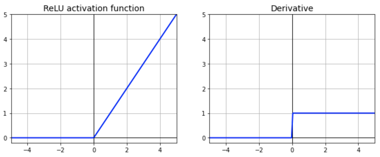
It is because we have one extra term to reduce the chance of having small gradient, as the error gradient can be directly passed to lower layers.

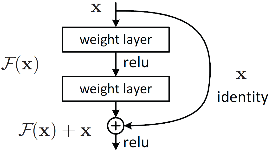
Besides ReLU and ResNet, Propose 3 more solutions to alleviate Vanishing Gradients.

• Xavier initialization

  • If weights in a DNN are too small to begin with, the signal strength shrinks during forward propagation. If the weights are too large, the signal strength will drive the network to saturation (going too small or too large). Xavier initialization is to ensure that the weights are just right to start with.

  • Method: Randomly initialize weights at layer $l$ with zero means and variance depending on the no. of neurons at Layer $l-1$ and Layer $l$ :

    $$\operatorname{Var}\left\{w_{i j}^{(l)}\right\}=\frac{2}{n_{l-1}+n_{l}}$$

• Batch norm

  • The idea is to bring the input to the activation function closer to 0 so that the gradient becomes non-zero.

  • Method: Normalizing the activation across the batch to have 0 mean and unit variance:

    • $\mu_{\mathcal{B}} \leftarrow \frac{1}{m} \sum_{i=1}^{m} x_{i} \quad$ // mini-batch mean
    • $\sigma_{\mathcal{B}}^{2} \leftarrow \frac{1}{m} \sum_{i=1}^{m}\left(x_{i}-\mu_{\mathcal{B}}\right)^{2}$ // mini-batch variance
    • $\widehat{x}_{i} \leftarrow \frac{x_{i}-\mu_{\mathcal{B}}}{\sqrt{\sigma_{\mathcal{B}}^{2}+\epsilon}}$ // normalize
    • $y_{i} \leftarrow \gamma \widehat{x}_{i}+\beta \equiv \mathrm{BN}_{\gamma, \beta}\left(x_{i}\right)$

  • During inference, we use the population statistics to perform the normalization:

  • $$y^{(k)}=B N_{\gamma^{(k)}, \beta^{(k)}}^{\inf }\left(x^{(k)}\right)=\frac{\gamma^{(k)}}{\sqrt{\operatorname{Var}\left[x^{(k)}\right]+\epsilon}}\left(x^{(k)}-E\left[x^{(k)}\right]\right)+\beta^{(k)}$$

    $E\left[x^{(k)}\right]=E_{B}\left[\mu_{B}^{(k)}\right]$ is the mean activation of a node for all batches $\operatorname{Var}\left[x^{(k)}\right]=\frac{m}{m-1} E_{B}\left[\sigma_{B}^{(k)^{2}}\right]$ is the activation variance of a node for all batches

• Layer norm

  • For RNNs, it is difficult to apply batch normalization. It is because the mini batches in RNN will have different input sequence size, it cannot give a fixed mean to favor batch normalization.
  • Layer norm is to apply normalization across the activation in a layer
  • 

Exploding Gradient (Concept)

Explain why Exploding Gradient happens.

When the initial weights generate some large loss, the gradients can accumulate during an update and result in very large gradients. The large gradients result in large updates to the network weights and leads to an unstable network. The parameters can sometimes become so large that they overflow and result in NaN values.

Another situation is when the weight vectors hit a cliff of the loss surface.

• The solution for this situation is to clip the gradient. clip_grad_nor

Almost no data per class (Concept)

Gradient-based methods require many examples per class and many iterations of network updates for the network to converge. With only a few examples per class, the network simply does no converge or will be severely overfitted. Propose a solution to solve this problem.

• Transfer Learning

Reference

Batch Normalization and ReLU for solving Vanishing Gradients

Why do ResNets avoid the vanishing gradient problem?