Paper Review - Denoising Diffusion Probabilistic Models (DDPM)

Update: A simplified DDPM pytorch implementation is available on https://github.com/vinesmsuic/simple-DDPM-annotated.

What is Diffusion?

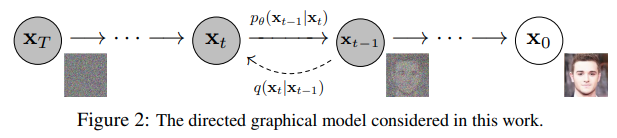
The essential idea is to systematically and slowly destroy structure in a data distribution through an iterative forward diffusion process which is fixed.

We then learn a reverse diffusion process that restores structure in data, yielding a highly flexible and tractable generative model of the data.

• Does it look like a Autoencoder approach?

DALLE2, MidJourney, Disco Diffusion, Stable Diffusion, Imagen are build on top of diffusion model.

DALLE1 is a Auto-regressive model.

In terms of photo-realism outputs, Diffusion models are better than GANs.

• Note: It is better if you understand VAE before studying Diffusion.

DDPM

Paper: Denoising Diffusion Probabilistic Models

The Annotated Diffusion Model

Lil’Log: What are Diffusion Models?

YouTube: Diffusion Models | Paper Explanation | Math Explained

YouTube: Diffusion models from scratch in PyTorch

YouTube: CVPR 2022 Tutorial on Denoising Diffusion-based Generative Modeling: Foundations and Applications

A (denoising) diffusion model is a neural network that learns to gradually denoise data starting from pure noise.

The set-up consists of 2 processes:

• Forward (Fixed)
  • Forward diffusion process $q$ : Gradually (regulated by a schedule) adds noise (sampled from a normal distribution) to an image until become pure noise
  • different amount of noise are applied in each timestep according to the schedule (different mean and variance)
• Reverse (Has to been Learned)
  • A Learned reverse denoising diffusion process $p_{\theta}$ : a neural network is trained to gradually denoise (remove a step of noise in each pass.) an image from pure noise to actual image.

By doing so, we can start with a completely random noise and let the model remove noise until we have a new image.

It’s a markov chain because it’s a sequence of stochastic events where each timestep depends on the previous timesteps.

• Note the latent states have the same dimensionality as the input image.

Training algorithm of DDPM

• 1: $x_0 \sim q(x_0)$: take a random sample $x_0$ from the real unknown and possibiliy complex data distribution $q(x_0)$
• 2: $t \sim \text{Uniform}(\{1,\dots,T\})$ : sample a noise level $t$ uniformally between $1$ and $T$ (i.e., a random time step)
• 3: $\epsilon\sim\mathcal{N}(0,I)$ : sample some noise (has same dimensionality as input data) from a gaussian distribution and corrupt the input by this noise at timestep $t$ , using the reparameterization trick $\sqrt{\bar\alpha_t}x_0 + \sqrt{1-\bar\alpha_t}\epsilon$
• 4: give the generated sample to the neural network to predict the noise based on the corrupted image $x_t$ and train the network
• 5: 1-4 are done on batches of data and optimize the network.

Something Important:

• Paper used T = 1000 (timestep = 1000), but the follow up papers are able to decrease this number.
• Images are scaled to inbetween [-1, 1] as to have the same range as the prior of a standard normal distribution $p(x_T) \sim \mathcal{N}(0,1)$ centered at 0 with variance of 1.

Inference algorithm of DDPM (Denoising)

As mentioned, generating new images from a diffusion model happens by reversing the diffusion process: we start from $T$, where we sample pure noise from a Gaussian distribution, and then use our neural network to gradually denoise it (using the conditional probability it has learned), until we end up at time step $t = 0$. By predicting the noise in each denoising step, we can get the less noisy image $x_{t-1}$ by predicting the mean and variance of the noise.

Ideally, we end up with an image that looks like it came from the real data distribution.

• 1: $x_T \sim \mathcal{N}(0,I)$: Draw samples from normal distribution $\mathcal{N}(0,I)$

• 2: for $t = T, \dots, 1$: for reverse timestep T to 1, at every step

• 3: draw white noise $z$ from normal distribution

  • If $t = 1$, we need not to add noise anymore.

• 4: Forming new sample with the mean of denoising model $\frac{1}{\sqrt{\alpha_t}}(x_t - \frac{1-\alpha_t}{\sqrt{1-\bar\alpha_t}}\epsilon_\theta(x_t,t))$ and then add the white noise $z$ rescaled with standard deviation $\sigma_t$.

DDPM From Math Perspective

Both the forward and reverse process are indexed by $t$ happen for some number of finite time steps $T$.

• Start with $t=0$, sample a real image $x_0$ from image distribution and apply some noise from a Gaussian distribution at each time step $t$, which is added to the image of the previous time step $t-1$.
  • $x_1$ will be 1st iteration of noise applied, $x_{42}$ will be 42th iteration of noise applied… The last step will be $x_t$.
• Given a large enough $T$, a well behaved schedule for adding noise at each time step, we get an isotropic Gaussian distribution at $t = T$ via a gradual process. (Isotropic means it looks the same in every direction)

We define function for Forward diffusion process $q(\mathrm{x}_t | x_{t-1})$ which means given an image with less noise at timestep $t-1$, we derive the image with little bit more noise at timestep $t$.

Then we also define function for reverse denoising diffusion process $p_\theta(\mathrm{x}_{t-1}|x_t)$ which means given an image with more noise at timestep $t$, we derive the image with less noise at timestep $t-1$. it is done by predicting the noise that was added to the image.

Forward Diffusion Process

From $x_0$ input image to a noisy version image at timestep $t$, it can be formulated as:

$$\mathrm{q}\left(\mathrm{x}_{1:T} \mid x_{0}\right) = \prod^T_{t=1}\mathrm{q}\left(\mathrm{x}_{t} \mid x_{t-1}\right)$$

The single forward diffusion process $q(\mathrm{x}_t | x_{t-1})$ can be formulated as $\mathcal{N}(z; \mu, \sigma)$:

$$\mathrm{q}\left(x_{t} \mid x_{t-1}\right)=\mathcal{N}\left(x_{t}; \sqrt{1-\beta_{t}} x_{t-1}, \beta_{t} I\right)$$

where

• $\mathcal{N}$ is the normal distribution
• $x_t$ is the output
• $\sqrt{1-\beta_{t}}x_{t-1}$ is the mean
• $\beta_{t} I$ is the variance
• $\beta$ is the scale at schedule

This means the sample $x_t$ is obtained by scaling the previous sample $x_{t-1}$ with $\sqrt{1-\beta_t}$ according to a variance schedule, then add independent and identically distributed Gaussian noise with square root of variance $\beta_t$ at timestep $t$.

$$x_t = \sqrt{1-\beta_t}x_{t-1} + \sqrt{\beta_t}\space \epsilon$$

where $\epsilon \sim \mathcal{N}(0, I)$ => sample from gaussian noise

DDPM used the linear schedule such that it will looks like this:

def linear_beta_schedule(timesteps):
 beta_start = 0.0001
 beta_end = 0.02
 return torch.linspace(beta_start, beta_end, timesteps)

• In later papers, Cosine schedule is used to replace linear schedule
  • Linear approach is sub-optimal because the last couple of timesteps already seems like complete noise and might be redundent. On the other hand, the information is destroyed too fast.
  • Cosine schedule solves both problems of the linear schedule

Since sum of gaussians is still a gaussian distribution, To apply multiple steps in one step, we can define:

• $\alpha_t = 1 - \beta_t$
• $\bar\alpha_t = \prod^t_{s=1} \alpha_s$
• Therefore at $t = 4$, $\alpha_4 = \alpha_1 \cdot \alpha_2 \cdot \alpha_3 \cdot \alpha_4$

Using the Reparameterization Trick $\mathcal{N}(\mu, \sigma^2) \rightarrow \mu+\sigma \cdot \epsilon$,

We get $\mathrm{q}\left(\mathrm{x}_{t} \mid x_{t-1}\right)=\mathcal{N}\left(x_{t}; \sqrt{1-\beta_{t}} x_{t-1}, \beta_{t} I\right) = \sqrt{1-\beta_{t}}x_{t-1} + \sqrt{\beta_t}\epsilon_{t-1}$

Sub $\alpha_t = 1 - \beta_t$ into the formula, we get

$x_t = \sqrt{1-\beta_{t}}x_{t-1} + \sqrt{\beta_t}\epsilon = \sqrt{\alpha_t} x_{t-1} + \sqrt{1-\alpha_t}\epsilon_{t-1}$.

Given $x_{t-1} = \sqrt{\alpha_{t-1}}x_{t-2} + \sqrt{1-\alpha_{t-1}}\epsilon_{t-2}$

We can represent $x_{t}$ as $\sqrt{\alpha_t\alpha_{t-1}} x_{t-2} + \sqrt{1-\alpha_t\alpha_{t-1}}\bar\epsilon_{t-2}$ , where $\bar\epsilon_{t-2}$ merge the two gaussians.

https://lilianweng.github.io/posts/2021-07-11-diffusion-models/#forward-diffusion-process

When we merge two Gaussians with different variance, $\mathcal{N}(0, \sigma^2_1 I)$ and $\mathcal{N}(0, \sigma^2_2 I)$,

the new distribution is $\mathcal{N}(0, (\sigma^2_1+\sigma^2_2) I)$ . With this property we can compute the merged standard deviation:

$$x_t = \sqrt{\alpha_t} x_{t-1} + \sqrt{1-\alpha_t}\epsilon_{t-1} = \sqrt{\alpha_t}(\sqrt{\alpha_{t-1}}x_{t-2} + \sqrt{1-\alpha_{t-1}}\epsilon_{t-2}) + \sqrt{1-\alpha_t}\epsilon_{t-1}$$

$$\sqrt{\alpha_t}(\sqrt{\alpha_{t-1}}x_{t-2} + \sqrt{1-\alpha_{t-1}}\epsilon_{t-2}) + \sqrt{1-\alpha_t}\epsilon_{t-1} =\sqrt{\alpha_t\alpha_{t-1}} x_{t-2} + (\sqrt{(\alpha_t)(1-\alpha_{t-1})}\epsilon_{t-2} + \sqrt{1-\alpha_t}\epsilon_{t-1} )$$

Forming new distribution $\mathcal{N}(0, (\sigma^2_1+\sigma^2_2) I)$,

$$(\sqrt{(\alpha_t)(1-\alpha_{t-1})}\epsilon_{t-2} + \sqrt{1-\alpha_t}\epsilon_{t-1} )= \sqrt{\sqrt{(\alpha_t)(1-\alpha_{t-1})}^2+\sqrt{1-\alpha_t}^2} \bar\epsilon_{t-2}$$

$$= \sqrt{a_t (1-a_{t-1}) + 1-a_t} \bar\epsilon_{t-2} = \sqrt{\cancel{a_t}- a_ta_{t-1} + 1 \cancel{-a_t}} \bar\epsilon_{t-2}$$

$$= \sqrt{1-\alpha_t\alpha_{t-1}}\bar\epsilon_{t-2}$$

Therefore we can represent $x_{t}$ as $\sqrt{\alpha_t\alpha_{t-1}} x_{t-2} + \sqrt{1-\alpha_t\alpha_{t-1}}\bar\epsilon_{t-2}$ , where $\bar\epsilon_{t-2}$ merge the two gaussians.

With this logic, we can represent $x_t$ as $\sqrt{\alpha_t\alpha_{t-1}\alpha_{t-2}} x_{t-3} + \sqrt{1-\alpha_t\alpha_{t-1}\alpha_{t-2}}\bar\epsilon_{t-3}$

Therefore, to sum up,

$$\sqrt{\alpha_{t} \alpha_{t-1} \ldots \alpha_{1} \alpha_{0}} x_{0}+\sqrt{1-\alpha_{t} \alpha_{t-1} \ldots \alpha_{1} \alpha_{0}} \bar\epsilon = \sqrt{\bar{\alpha}_t x_0} + \sqrt{1-\bar{\alpha}_t}\bar\epsilon$$

and rewrite as:

$$\mathrm{q}\left(x_{t} \mid x_{0}\right)=\mathcal{N}\left(x_{t}; \sqrt{\bar\alpha_t} x_{0}, (1-\bar\alpha_t) I\right)$$

So to do sampling we can simply do

$$x_t = \sqrt{\bar{\alpha}_t}x_0 + \sqrt{(1-\bar{\alpha}_t)}\epsilon$$

where $\epsilon \sim \mathcal{N}(0, I)$ => sample from gaussian noise

# Define beta schedule
T = 250
betas = linear_beta_schedule(timesteps=T)

# calculate alphas
alphas = 1. - betas
alphas_cumprod = torch.cumprod(alphas, axis=0)


alphas_cumprod_prev = F.pad(alphas_cumprod[:-1], (1, 0), value=1.0)
sqrt_recip_alphas = torch.sqrt(1.0 / alphas)

# calculations for diffusion q(x_t | x_{t-1}) and others
sqrt_alphas_cumprod = torch.sqrt(alphas_cumprod)
sqrt_one_minus_alphas_cumprod = torch.sqrt(1. - alphas_cumprod)

# calculations for posterior q(x_{t-1} | x_t, x_0)
posterior_variance = betas * (1. - alphas_cumprod_prev) / (1. - alphas_cumprod)

# Get the indexed term from the list
# https://github.com/pytorch/pytorch/issues/15245 Gather backward is faster than integer indexing on GPU
def extract(a, t, x_shape):
    batch_size = t.shape[0]
    out = a.gather(-1, t.cpu())
    return out.reshape(batch_size, *((1,) * (len(x_shape) - 1))).to(t.device)

# forward diffusion (using the nice property alpha)
def q_sample(x_start, t, noise=None):
    if noise is None:
        noise = torch.randn_like(x_start)
	
    # \sqrt{\bar\alpha_t}
    sqrt_alphas_cumprod_t = extract(sqrt_alphas_cumprod, t, x_start.shape)
    
    # \sqrt{(1-\bar\alpha_t)}
    sqrt_one_minus_alphas_cumprod_t = extract(
        sqrt_one_minus_alphas_cumprod, t, x_start.shape
    )
	
    # \mathcal{N}\left(x_{t}; \sqrt{\bar\alpha_t} x_{0}, (1-\bar\alpha_t) I\right)
    # N(mean, var) * (1-alpha_cumprod) = N(mean, (1-alpha_cumprod) * var)
    return sqrt_alphas_cumprod_t * x_start + sqrt_one_minus_alphas_cumprod_t * noise

So the forward process looks like this:

But what is really happening?

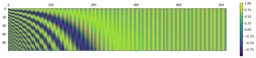
• At small t, most of the low frequency contents are not perturbed by the noise, but high frequency content are being perturbed.
• At bigger t, low frequency contents are also perturbed.
• At the end of forward process, we get rid of the both low and high frequency contents of image.

Parametrized Reverse Denoising Diffusion Process

To reverse the process, the intuitive idea is to find $\mathrm{q}\left(x_{t-1} \mid x_{t}\right)$.

However, $q\left(\mathbf{x}_{t-1} \mid \mathbf{x}_t\right) \propto q\left(\mathbf{x}_{t-1}\right) q\left(\mathbf{x}_t \mid \mathbf{x}_{t-1}\right)$ is intractable. Instead, we can approximate $\mathrm{q}\left(x_{t-1} \mid x_{t}\right)$ using a Normal distribution if $\beta_t$ is small in each forward diffusion step.

Generating new images from a diffusion model happens by reversing the diffusion process: we start from $T$, where we sample pure noise from a Gaussian distribution, and then use our neural network to gradually denoise it (using the conditional probability it has learned), until we end up at time step $t = 0$. Ideally, we end up with an image that looks like it came from the real data distribution.

From pure noise / noisy image $x_t$ to original image $x_0$ or less noisy image at timestep $t$, it can be formulated as:

$$p_{\theta}(x_{0:T})=p(x_T)\prod^T_{t=1}p_{\theta}(x_{t-1}|x_t)$$

$$p(x_T) = \mathcal{N}(x_T; 0, I)$$

The single reverse denoising diffusion process $p(\mathrm{x}_{t-1}|x_t)$ can be formulated as $\mathcal{N}(z; \mu, \sigma)$:

$$p_\theta\left(x_{t-1} \mid x_{t}\right)=\mathcal{N}\left(x_{t-1} ; \mu_{\theta}\left(x_{t}, t\right), \Sigma_{\theta}\left(x_{t}, t\right)\right)$$

where

• $\mathcal{N}$ is the normal distribution
• $\mu_{\theta}$ parametrize the mean
• $\sum_\theta$ parameterize the variance

We can derive a slightly less denoised image $\mathbf{x}_{t-1 }$ by plugging in the reparametrization of the mean and variance.

We need a trainable neural network to represent a (conditional) probability distribution of the backward process. We want to learn 2 parameters:

• a mean parametrized by $\mu_{\theta}\left(x_{t}, t\right)$
• a variance parameterized by $\Sigma_{\theta}\left(x_{t}, t\right)$

However, DDPM authors decided to keep the variance fixed, and let the neural network only learn (represent) the mean $\mu_\theta$ of the conditional probability distribution.

$$p\left(x_{t-1} \mid x_{t}\right)=\mathcal{N}\left(x_{t-1} ; \mu_{\theta}\left(x_{t}, t\right), \beta_t I\right)$$

where a linear schedule is used

Later in the Improved diffusion models paper, a neural network also learns the variance of this backward process, besides the mean.

By predicting the mean of noise, we can know the Noise of the image.

In order to get the exact image, we simply get $x_{t-1} \approx x_t - \text{noise}$.

The predicted mean of noise:

$$\mu_{\theta}(x_{t}, t) = \tilde{\mu}_{t}(x_t, \frac{1}{\sqrt{\alpha_t}}(x_t - {\sqrt{1-\overline{\alpha}_t}}\epsilon_{\theta}(x_t)))$$

$$= \frac{1}{\sqrt{\alpha_t}}(x_t - \frac{\beta_t}{\sqrt{1-\overline{\alpha}_t}}\epsilon_{\theta}(x_t, t)) = \frac{1}{\sqrt{\alpha_t}}(x_t - \frac{\beta_t \epsilon_{\theta}(x_t, t)}{\sqrt{1-\overline{\alpha}_t}})$$

# Define beta schedule
T = 300
betas = linear_beta_schedule(timesteps=T)

# calculate alphas
alphas = 1. - betas
alphas_cumprod = torch.cumprod(alphas, axis=0)


alphas_cumprod_prev = F.pad(alphas_cumprod[:-1], (1, 0), value=1.0)
sqrt_recip_alphas = torch.sqrt(1.0 / alphas)

# calculations for diffusion q(x_t | x_{t-1}) and others
sqrt_alphas_cumprod = torch.sqrt(alphas_cumprod)
sqrt_one_minus_alphas_cumprod = torch.sqrt(1. - alphas_cumprod)

# calculations for posterior q(x_{t-1} | x_t, x_0)
posterior_variance = betas * (1. - alphas_cumprod_prev) / (1. - alphas_cumprod)

# Get the indexed term from the list
# https://github.com/pytorch/pytorch/issues/15245 Gather backward is faster than integer indexing on GPU
def extract(a, t, x_shape):
    batch_size = t.shape[0]
    out = a.gather(-1, t.cpu())
    return out.reshape(batch_size, *((1,) * (len(x_shape) - 1))).to(t.device)

@torch.no_grad()
def p_sample(model, x, t, t_index):
   	"""
    Sample from the model. Mean is predicted, Variance is fixed in this example
    """
    betas_t = extract(betas, t, x.shape)
    sqrt_one_minus_alphas_cumprod_t = extract(
        sqrt_one_minus_alphas_cumprod, t, x.shape
    )
    sqrt_recip_alphas_t = extract(sqrt_recip_alphas, t, x.shape)
    
    # Use our model (noise predictor) to predict the mean
    model_mean = sqrt_recip_alphas_t * (
        x - betas_t * model(x, t) / sqrt_one_minus_alphas_cumprod_t
    )

    if t_index == 0:
        return model_mean
    else:
        posterior_variance_t = extract(posterior_variance, t, x.shape)
        noise = torch.randn_like(x)
        # x_{t-1} sample is generated
        image = model_mean + torch.sqrt(posterior_variance_t) * noise 
        return image

To denoise from timestep $T$ to 0 and get a clear image, we iteratively do the denoising step.

@torch.no_grad()
def p_sample_loop(model, shape):
    device = next(model.parameters()).device

    b = shape[0]
    # start from pure noise (for each example in the batch)
    img = torch.randn(shape, device=device)
    imgs = []
    
    for i in tqdm(reversed(range(0, timesteps)), desc='sampling loop time step', total=timesteps):
        img = p_sample(model, img, torch.full((b,), i, device=device, dtype=torch.long), i)
        imgs.append(img.cpu().numpy())
    return imgs

@torch.no_grad()
def sample(model, image_size, batch_size=16, channels=3):
    return p_sample_loop(model, shape=(batch_size, channels, image_size, image_size))

The above code return the image output in all the denoising steps. Alternatively we can modify the code to send only the last step.

@torch.no_grad()
def p_sample_loop_last(model, shape):
    device = next(model.parameters()).device

    b = shape[0]
    # start from pure noise (for each example in the batch)
    img = torch.randn(shape, device=device)
    imgs = []
    
    final_img = None
    for i in tqdm(reversed(range(0, timesteps)), desc='sampling loop time step', total=timesteps):
        img = p_sample(model, img, torch.full((b,), i, device=device, dtype=torch.long), i)
    final_img = img.cpu().numpy()
    return final_img

Recall what we understood in the forward process. In large timesteps, the low frequency components are hidden, and in less timestep, the high-frequency contents are hidden.

Therefore, in the reverse process, we can make a trade-off between content detail with the weighting.

• Low frequency content responses to the main content of the image
• High-frequency content responses to the low-level fine details

Therefore the noise schedule can play a huge role here.

Objective function of Diffusion

The loss function is simply the negative log likelihood

$$-\log(p_\theta(x_0))$$

However, $p_\theta(x_0)$ is not nicely computable as it depend all other timesteps coming before $x_0$ (i.e. $x_T, ..., x_1$)

As a solution we can compute the variational lower bound, that is commonly used for training Variational Autoencoder. We write this formula:

$$-\log(p_\theta(x_0)) \leq -\log(p_\theta(x_0)) + D_{KL}(q(x_{1:T}|x_0)||p_\theta(x_{1:T}|x_0))$$

• Note the KL divergence $D_{KL}(q(x_{1:T}|x_0)||p_\theta(x_{1:T}|x_0))$ is something non-negative.

But its still not computable as the $-\log(p_\theta(x_0))$ still exists; so we need to further rewrite the formula:

We can rewrite the KL divergence such that

$$D_{KL}(q(x_{1:T}|x_0)||p_\theta(x_{1:T}|x_0)) = \log(\frac{q(x_{1:T})|x_0}{p_\theta(x_{1:T}|x_0)})$$

Then bayesian rule:

$$\log(\frac{q(x_{1:T})|x_0}{p_\theta(x_{1:T}|x_0)}) = \frac{p_\theta(x_0|x_{1:T})p_\theta(x_{1:T})}{p_\theta(x_0)}$$

$$\frac{p_\theta(x_0|x_{1:T})p_\theta(x_{1:T})}{p_\theta(x_0)} = \frac{p_\theta(x_0,x_{1:T})}{p_\theta(x_0)} = \frac{p_\theta(x_{0:T})}{p_\theta(x_0)}$$

Turn it into log and move it around

$$\frac{p_\theta(x_{0:T})}{p_\theta(x_0)} = \log(\frac{q(x_{1:T}|x_0)}{\frac{p_\theta(x_{0:T})}{p_\theta(x_0)}}) = \log(\frac{q(x_{1:T}|x_0)p_\theta(x_0)}{p_\theta(x_{0:T})})$$

$$\log(\frac{q(x_{1:T}|x_0)p_\theta(x_0)}{p_\theta(x_{0:T})}) = \log(\frac{q(x_{1:T}|x_0)}{p_\theta(x_{0:T})}) + \log(p_\theta(x_0))$$

So we get

$$-\log(p_\theta(x_0)) \leq -\log(p_\theta(x_0)) + \log(\frac{q(x_{1:T}|x_0)}{p_\theta(x_{0:T})}) + \log(p_\theta(x_0))$$

which the two $\log(p_\theta(x_0))$ terms can be cancelled each other and become the variational lower bound that we want to minimize.

$$-\log(p_\theta(x_0)) \leq \log(\frac{q(x_{1:T}|x_0)}{p_\theta(x_{0:T})})$$

where

• $q(x_{1:T}|x_0)$ is the forward process (Given initial image $x_0$ find $x_{1:T}$)
  • which can be reformulated as $\prod^T_{t=1}\mathrm{q}\left(\mathrm{x}_{t} \mid x_{t-1}\right)$
• $p_\theta(x_{0:T})$ is the reverse process (From noisy image to initial image)
  • which can be reformulated as $p(x_T)\prod^T_{t=1}p_{\theta}(x_{t-1}|x_t)$

$$-\log(p_\theta(x_0)) \leq \log(\frac{\prod^T_{t=1}\mathrm{q}\left(\mathrm{x}_{t} \mid x_{t-1}\right)}{p(x_T)\prod^T_{t=1}p_{\theta}(x_{t-1}|x_t)})$$

we can extract the computable term $p(x_T)$ from $\log(\frac{\prod^T_{t=1}\mathrm{q}\left(\mathrm{x}_{t} \mid x_{t-1}\right)}{p(x_T)\prod^T_{t=1}p_{\theta}(x_{t-1}|x_t)})$

$$\log(\frac{\prod^T_{t=1}\mathrm{q}\left(\mathrm{x}_{t} \mid x_{t-1}\right)}{p(x_T)\prod^T_{t=1}p_{\theta}(x_{t-1}|x_t)}) = \log(\frac{\prod^T_{t=1}\mathrm{q}\left(\mathrm{x}_{t} \mid x_{t-1}\right)}{\prod^T_{t=1}p_{\theta}(x_{t-1}|x_t)}) - \log(p(x_T))$$

Bring out the product term to become the sum (log rules)

$$\log(\frac{\prod^T_{t=1}\mathrm{q}\left(\mathrm{x}_{t} \mid x_{t-1}\right)}{\prod^T_{t=1}p_{\theta}(x_{t-1}|x_t)}) - \log(p(x_T)) = - \log(p(x_T)) + \sum^T_{t=1}\log(\frac{q(x_t|x_{t-1})}{p_\theta(x_{t-1}|x_t)})$$

The author did a little trick to move the parametrized term. First split up the first term of the summation:

$$- \log(p(x_T)) + \sum^T_{t=1}\log(\frac{q(x_t|x_{t-1})}{p_\theta(x_{t-1}|x_t)})=- \log(p(x_T)) + \sum^T_{t=2}\log(\frac{q(x_t|x_{t-1})}{p_\theta(x_{t-1}|x_t)}) + \log(\frac{q(x_1|x_{0})}{p_\theta(x_{0}|x_1)})$$

By the bayes rule $q(x_t|x_{t-1}) = \frac{q(x_{t-1}|x_{t})q(x_t)}{q(x_{t-1})}$ , we get the three terms with high variance (We dont know where the noise image came from). Therefore we could reduce the variance by conditioning $x_0$ (Given the initial noise-free picture) such that $\frac{q(x_{t-1}|x_{t})q(x_t)}{q(x_{t-1})} \Rightarrow \frac{q(x_{t-1}|x_{t}, x_0)q(x_t|x_0)}{q(x_{t-1}|x_0)}$

$$q(x_t|x_{t-1}) = \frac{q(x_{t-1}|x_{t})q(x_t)}{q(x_{t-1})} \Rightarrow \frac{q(x_{t-1}|x_{t}, x_0)q(x_t|x_0)}{q(x_{t-1}|x_0)}$$

Plugging this term $q(x_t|x_{t-1}) = \frac{q(x_{t-1}|x_{t}, x_0)q(x_t|x_0)}{q(x_{t-1}|x_0)}$ into $- \log(p(x_T)) + \sum^T_{t=2}\log(\frac{q(x_t|x_{t-1})}{p_\theta(x_{t-1}|x_t)}) + \log(\frac{q(x_1|x_{0})}{p_\theta(x_{0}|x_1)})$, We have

$$- \log(p(x_T)) + \sum^T_{t=2}\log(\frac{q(x_{t-1}|x_{t}, x_0)q(x_t|x_0)}{p_\theta(x_{t-1}|x_t)q(x_{t-1}|x_0)}) + \log(\frac{q(x_1|x_{0})}{p_\theta(x_{0}|x_1)})$$

Split up the summation part

$$= - \log(p(x_T)) + \sum^T_{t=2}\log(\frac{q(x_{t-1}|x_{t}, x_0)}{p_\theta(x_{t-1}|x_t)}) + \sum^T_{t=2}\log(\frac{q(x_t|x_0)}{q(x_{t-1}|x_0)}) + \log(\frac{q(x_1|x_{0})}{p_\theta(x_{0}|x_1)})$$

The term $\sum^T_{t=2}\log(\frac{q(x_t|x_0)}{q(x_{t-1}|x_0)})$ can be simplified as

$$\sum^T_{t=2}\log(\frac{q(x_t|x_0)}{q(x_{t-1}|x_0)}) = \log(\prod^T_{t=2}\frac{q(x_t|x_0)}{q(x_{t-1}|x_0)}) = \log(\frac{q(x_T|x_0)}{q(x_{1}|x_0)})$$

Because e.g. Let $T = 5$:

$$\sum^5_{t=2}\log(\frac{q(x_t|x_0)}{q(x_{t-1}|x_0)}) = \log(\prod^5_{t=2}\frac{q(x_t|x_0)}{q(x_{t-1}|x_0)}) = \log(\frac{\cancel{q(x_2|x_0)q(x_3|x_0)q(x_4|x_0)}q(x_5|x_0)}{q(x_{1}|x_0)\cancel{q(x_{2}|x_0)q(x_{3}|x_0)q(x_{4}|x_0)}}) = \log(\frac{q(x_5|x_0)}{q(x_{1}|x_0)})$$

So we get

$$- \log(p(x_T)) + \sum^T_{t=2}\log(\frac{q(x_{t-1}|x_{t}, x_0)}{p_\theta(x_{t-1}|x_t)}) + \log(\frac{q(x_T|x_0)}{q(x_{1}|x_0)}) + \log(\frac{q(x_1|x_{0})}{p_\theta(x_{0}|x_1)})$$

extract the terms using log rules and found we can cancel some terms.

$$= - \log(p(x_T)) + \sum^T_{t=2}\log(\frac{q(x_{t-1}|x_{t}, x_0)}{p_\theta(x_{t-1}|x_t)}) + \log(q(x_T|x_0)) \cancel{-\log(q(x_{1}|x_0)) + \log(q(x_1|x_{0}))} - \log(p_\theta(x_{0}|x_1))$$

$$= - \log(p(x_T)) + \sum^T_{t=2}\log(\frac{q(x_{t-1}|x_{t}, x_0)}{p_\theta(x_{t-1}|x_t)}) + \log(q(x_T|x_0)) - \log(p_\theta(x_{0}|x_1))$$

Fuse the term $- \log(p(x_T))$ and $+\log(q(x_T|x_0))$ using log rule to form $\log{(\frac{q(x_T|x_0)}{p(x_T)})}$

$$= \log{(\frac{q(x_T|x_0)}{p(x_T)})} + \sum^T_{t=2}\log(\frac{q(x_{t-1}|x_{t}, x_0)}{p_\theta(x_{t-1}|x_t)}) - \log(p_\theta(x_{0}|x_1))$$

Convert $\log{(\frac{q(x_T|x_0)}{p(x_T)})}$ and $\sum^T_{t=2}\log(\frac{q(x_{t-1}|x_{t}, x_0)}{p_\theta(x_{t-1}|x_t)})$ into KL Divergence terms, our objective is:

$$L=\mathbb{E}_q[\underbrace{D_{\mathrm{KL}}\left(q\left(\mathbf{x}_T \mid \mathbf{x}_0\right) \| p\left(\mathbf{x}_T\right)\right)}_{L_T}+\sum_{t>1} \underbrace{D_{\mathrm{KL}}\left(q\left(\mathbf{x}_{t-1} \mid \mathbf{x}_t, \mathbf{x}_0\right) \| p_\theta\left(\mathbf{x}_{t-1} \mid \mathbf{x}_t\right)\right)}_{L_{t-1}} \underbrace{\left.-\log p_\theta\left(\mathbf{x}_0 \mid \mathbf{x}_1\right)\right)}_{L_0}]$$

$$D_{KL}(q(x_T|x_0)||p(x_T)) + \sum^T_{t=2} D_{KL} (q(x_{t-1}|x_{t}, x_0) || p_\theta(x_{t-1}|x_t)) - \log(p_{\theta}(x_0|x_1))$$

Note the first term $D_{KL}(q(x_T|x_0)||p(x_T))$ can be dropped because it has no learnable parameters, and the term will be small. It is simply the KL divergence from the diffusion kernel in the last step $(x_T|x_0)$ to the base distribution $x_T$. The $(x_T|x_0)$ is converge to a standard normal distribution, which is the same distribution as $x_T$. Therefore after dropping the first term we have:

$$\sum^T_{t=2} D_{KL} (q(x_{t-1}|x_{t}, x_0) || p_\theta(x_{t-1}|x_t)) - \log(p_{\theta}(x_0|x_1))$$

Given $p\left(x_{t-1} \mid x_{t}\right)=\mathcal{N}\left(x_{t-1} ; \mu_{\theta}\left(x_{t}, t\right), \beta I\right)$ <= In DDPM the variance is fixed, and

$q(x_{t-1}|x_{t}, x_0) = \mathcal{N}(x_{t-1}, \tilde{\mu}_t(x_t, x_0), \tilde{\beta}_tI)$ <= We skip the explaination but $q(x_{t-1}|x_{t}, x_0)$ is the tractable posterior distribution.

Note

• $\tilde{\mu}_t(x_t, x_0) = \frac{\sqrt{\alpha_t}(1-\bar{\alpha}_{t-1})}{1-\bar{\alpha}_t}x_t + \frac{\sqrt{\bar{\alpha}_{t-1}}\beta_t}{1-\bar{\alpha}_t}x_0$
• $\tilde{\beta}_tI = \frac{1-\bar{\alpha}_{t-1}}{1-\bar{\alpha}_{t}} \cdot \beta_t$

Recall: to apply multiple step into one step,

$$x_t = \sqrt{\bar{\alpha}_t x_0} + \sqrt{1-\bar{\alpha}_t}\epsilon$$

Therefore

$$x_0 = \frac{1}{\sqrt{\bar{\alpha}}_t}(x_t - \sqrt{1-\bar{\alpha}_t}\epsilon)$$

Plugging $x_0 = \frac{1}{\sqrt{\bar{\alpha}}_t}(x_t - \sqrt{1-\bar{\alpha}_t}\epsilon)$ into $\tilde{\mu}_t(x_t, x_0) = \frac{\sqrt{\alpha_t}(1-\bar{\alpha}_{t-1})}{1-\bar{\alpha}_t}x_t + \frac{\sqrt{\bar{\alpha}_{t-1}}\beta_t}{1-\bar{\alpha}_t}x_0$ , we get:

$$\tilde{\mu}_t(x_t, x_0) = \frac{\sqrt{\alpha_t}(1-\bar{\alpha}_{t-1})}{1-\bar{\alpha}_t}x_t + \frac{\sqrt{\bar{\alpha}_{t-1}}\beta_t}{1-\bar{\alpha}_t}\frac{1}{\sqrt{\bar{\alpha}}_t}(x_t - \sqrt{1-\bar{\alpha}_t}\epsilon)$$

And end up getting the formula as the predicted noise.

$$\tilde{\mu}_t(x_t, x_0) = \frac{1}{\sqrt{\alpha_t}}(x_t - \frac{\beta_t}{\sqrt{1-\bar{\alpha}_t}}\epsilon)$$

Therfore we can predict the noise with the neural network:

$$\mu_{\theta}(x_{t}, t) = \frac{1}{\sqrt{\alpha_t}}(x_t - \frac{\beta_t}{\sqrt{1-\overline{\alpha}_t}} \epsilon_{\theta}(x_t, t))$$

The DDPM author declared the MSE loss between the actual noise and the predicted noise.

$$\mathcal{L}_{t-1} = \frac{1}{2\sigma^2_t}||\tilde{\mu}_t(x_t, x_0) - \mu_{\theta}(x_{t}, t)||^2$$

$$\mathcal{L}_{t-1} = \frac{1}{2\sigma^2_t}||\frac{1}{\sqrt{\alpha_t}}(x_t - \frac{\beta_t}{\sqrt{1-\bar{\alpha}_t}}\epsilon) - \frac{1}{\sqrt{\alpha_t}}(x_t - \frac{\beta_t}{\sqrt{1-\bar{\alpha}_t}}\epsilon_{\theta}(x_t,t))||^2$$

Which are completely the same except the epsilon term. Through simplification, we get

$$\mathcal{L}_{t-1} = \frac{\beta_t^2}{2\sigma^2_t \alpha_t(1-\hat{\alpha}_t)}||\epsilon - \epsilon_\theta(x_t, t)||^2$$

we can replace the scalar term with a time dependant lambda value:

$$\mathcal{L}_{t-1} = \lambda_t||\epsilon - \epsilon_\theta(x_t, t)||^2$$

where the time dependant $\lambda_t$ ensures that the training objective is weighted properly for the maximum data likelihood training. However, this weight is often very large for small $t$ 's, and very small for large $t$’s.

… And then the author found out ignore the scaling term (put $\lambda_t = 1$) would result a better quality. Therefore we get:

$$\mathcal{L}_{t-1} = ||\epsilon - \epsilon_\theta(x_t, t)||^2$$

Replugging the term into $\sum^T_{t=2} D_{KL} (q(x_{t-1}|x_{t}, x_0)$:

$$\mathcal{L}_{VLB} = \sum^T_{t=2} ||\epsilon - \epsilon_\theta(x_t, t)||^2 - \log(p_{\theta}(x_0|x_1))$$

As at sampling time $t=1$ we dont noise to it, we can drop the $- \log(p_{\theta}(x_0|x_1)$ term as well So Finally:

$$\mathcal{L}_{simple} = \mathbb{E}_{t,x_0,\epsilon}[||\epsilon - \epsilon_\theta(x_t, t)||^2]$$

So that’s way basically in implementation, we want to compute a MSE loss (or any loss) between the real noise and the predicted noise.

def p_losses(denoise_model, x_start, t, noise=None, loss_type="l1"):
    if noise is None:
        noise = torch.randn_like(x_start)

    x_noisy = q_sample(x_start=x_start, t=t, noise=noise)
    predicted_noise = denoise_model(x_noisy, t)

    if loss_type == 'l1':
        loss = F.l1_loss(noise, predicted_noise)
    elif loss_type == 'l2':
        loss = F.mse_loss(noise, predicted_noise)
    elif loss_type == "huber":
        loss = F.smooth_l1_loss(noise, predicted_noise)
    else:
        raise NotImplementedError()

    return loss

Components of a Diffusion model

We will need mainly 3 components:

• A UNet model that predicts the noise in an image
• Noise Scheduler that sequentially adds noise
• A way to encode the current timestep

Generally we want to use a network that is similar to Autoencoder. we want to have “bottleneck” layer in between the encoder and decoder. The encoder first encodes an image into a smaller hidden representation called the “bottleneck”, and the decoder then decodes that hidden representation back into an actual image. This forces the network to only keep the most important information in the bottleneck layer.

• DDPM authors used a U-Net, similar to an unmasked PixelCNN++ with group normalization throughout
  • bottleneck, residual connections between encoder and decoder (greatly improving gradient flow)
  • Attention, ConvNext
  • Sinusoidal embedding from Transformer is used to project into each residual block because to create a denoising schedule that match the noising schedule in the forward process
  • UNet is a segmentation network that gives an output dimension same as input dimension.
• The model take a noisy image with 3 color channels as inputs, and predict the noise in the image
  • That means the model learns the mean (and variance) of the gaussian distribution of the images
    • Known as denoising score matching

• Timestep encoding is used to encode the timestep such that the model knows which timestep it is in.
  • To encode the timestep, we can use sinusoidal embedding (hand-crafted) or some other positional embeddings (learned from data)
  • The key idea is that each position has a unique positional vector