Advanced Techniques of Diffusion Models

Advanced Techniques: Accelerated Sampling, Conditional Generation

Advanced Techniques of Diffusion Models: Accelerated Sampling, Conditional Generation

How to accelerate the sampling process

What makes a good generative model?

• Fast sampling from the generative model
• Model coverage/ diversity (generative model capture most of the major modes of the data distribution)
• High quality / high fidelity samples

	GANs	VAEs, Normaling Flows	Diffusion Models
Fast Sampling	✅	✅	❌
Mode coverage/ diversity	❌	✅	✅
High quality samples	✅	❌	✅

Accelerating Diffusion Models

Naive accelerate methods, such as reducing diffusion timesteps in training or sampling every k timestep in inference, lead to immediate worse performance.

Advanced forward process

• Does the noise schedule have to be predefined?
• Does the forward process of DDPM has to be a Markovian process?
• Is there any faster mixing diffusion process?

Covering: VDM, DDIM, Critically-damped Langevin diffusion

Variational Diffusion Models

Variational Diffusion Models: https://arxiv.org/abs/2107.00630

Learnable diffusion process => Include Learnable Parameters in the encoder

• Given the forward process $q(x_t|x_0) = \mathcal{N}(x_t; \sqrt{\bar{\alpha_t}}x_0, (1-\bar{\alpha}_t)\mathbf{I})$
• Directly parametrize the variance through a learned function $\gamma_\eta$:
  • $(1 - \bar \alpha_t) = \text{sigmoid}(\gamma_\eta(t))$
  • $(\gamma_\eta(t))$ is a monotonic MLP
    • Strictly positive weights and monotonic activations (e.g. sigmoid)

New parametrization of training objectives

We call that we learned that the diffusion models can be interpreted from the perspective of SDE (Stochastic Differential Equation), and we learned the connection between diffusion models and denoising score matching. This implies that the diffusion models can also be defined in the continuous-time setting.

• Optimizing variational upper bound of diffusion models can be simplified to the following training objective:
  • $\mathcal{L}_T=\frac{T}{2} \mathbb{E}_{\mathrm{x}_0, \epsilon, t}\left[\left(\exp \left(\gamma_\eta(t)-\gamma_\eta(t-1)\right)-1\right)\left\|\epsilon-\epsilon_\theta\left(\mathbf{x}_t, t\right)\right\|_2^2\right]$
• Letting $T \rightarrow \infty$ leads to variation upper bound in continuous-time
  • When $T \rightarrow \infty$ , we have infinity amount of diffusion steps which corresponds to a continuous time setting and then the variantion upper bound can be derived
  • $\mathcal{L}_\infty=\frac{1}{2} \mathbb{E}_{\mathrm{x}_0, \epsilon, t}\left[\gamma_\eta'(t)\|\epsilon-\epsilon_\theta(\mathbf{x}_t, t)\|_2^2\right], \quad \gamma_\eta'(t) = d\gamma_\eta(t)/dt$
• It is shown to be only related to the signal-to-noise ration $SNR(t) = \bar\alpha_t/(1-\bar\alpha_t) = \exp (-\gamma_\eta(t))$ at endpoints, invarient to the noise schedule in-between. It means we only need to optimize the SNR at the beginning and the end of the forward process
• The continuous-time noise schedule can be learned to minimize the variance of the training objective for faster training.

SOTA likelihood estimation (significant improvements in log-likelihoods)

• Appending Fourier features to the input of U-Net
  • $f^n_{i,j,k} = \sin(x_{i,j,k}2^n\pi), g^n_{i,j,k} = \cos (x_{i,j,k}2^n\pi), n = 7, 8$
• Hypothesis: To get good likelihoods, the model need to modeling all the bits (details in the input signal, both perceptual and inperceptual). But neural nets are usually bad at modeling small changes to inputs.

Denoising Diffusion Implicit Models (DDIM)

Denoising Diffusion Implicit Models: https://arxiv.org/abs/2010.02502

Non-Markovian Diffusion Process

• Define a family of non-Markovian diffusion processes and corresponding reverse processes.
• The process is designed such that the model can be optimized by the same surrogate objective as the original diffusion model.
  • Recall the objective of the original diffusion model: $\mathcal{L}_{simple}(\theta) := \mathbb{E}_{t,x_0,\epsilon}[||\epsilon-\epsilon_\theta(\sqrt{\bar\alpha_t}x_0+\sqrt{1-\bar\alpha_t}\epsilon, t)||^2]$
  • Therefore can take a pretrained diffusion model but with more choices of sampling procedure.

To Define the non-Markovian forward process

Recall the Objective of diffusion models:

$$L=\mathbb{E}_q[\underbrace{D_{\mathrm{KL}}\left(q\left(\mathbf{x}_T \mid \mathbf{x}_0\right) \| p\left(\mathbf{x}_T\right)\right)}_{L_T}+\sum_{t>1} \underbrace{D_{\mathrm{KL}}\left(q\left(\mathbf{x}_{t-1} \mid \mathbf{x}_t, \mathbf{x}_0\right) \| p_\theta\left(\mathbf{x}_{t-1} \mid \mathbf{x}_t\right)\right)}_{L_{t-1}} \underbrace{\left.-\log p_\theta\left(\mathbf{x}_0 \mid \mathbf{x}_1\right)\right)}_{L_0}]$$

KL divergence in the variational upper bound can be written as

$$\mathcal{L}_{t-1}= D_{KL} (q(x_{t-1}|x_{t}, x_0) || p_\theta(x_{t-1}|x_t)) = \mathbb{E}_q[\frac{1}{2\sigma^2_t}||\tilde{\mu}_t(x_t, x_0)-\mu_\theta(x_t, t)||^2] + C$$

• $q(x_{t-1}|x_t, x_0)$ is the posterior distribution
• $p_\theta(x_{t-1}|x_t)$ is the denoising distribution
• Since both distributions are Gaussian distributions with the same variance $\sigma_t^2$, this can be written as the L2 distance between the mean of the 2 distributions and times a constant $\frac{1}{2\sigma^2_t}$
  • $\mathbb{E}_q[\frac{1}{2\sigma^2_t}||\tilde{\mu}_t(x_t, x_0)-\mu_\theta(x_t, t)||^2]$

https://vinesmsuic.github.io/paper-ddpm/#Objective-function-of-Diffusion

Recall the two mean functions $\tilde{\mu}_t(x_t, x_0)$, $\mu_\theta(x_t, t)$ have been parametrized by simple linear combination of $x_t$

• $\tilde{\mu}_t(x_t, x_0) = \frac{1}{\sqrt{1-\beta_t}}(x_t - \frac{\beta_t}{\sqrt{1-\bar\alpha_t}}\epsilon)$
• $\mu_\theta(x_t, t) = \frac{1}{\sqrt{1-\beta_t}}(x_t - \frac{\beta_t}{\sqrt{1-\bar\alpha_t}}\epsilon_\theta(x_t, t))$

Then we can rewrite $\mathbb{E}_q[\frac{1}{2\sigma^2_t}||\tilde{\mu}_t(x_t, x_0)-\mu_\theta(x_t, t)||^2] + C$ to

$$\mathbb{E}_{x_0\sim q(x_0), \epsilon\sim\mathcal{N}(0,\mathbf{I})} [\lambda_t||\epsilon - \epsilon_\theta(\sqrt{\bar\alpha_t}x_0 + \sqrt{1-\bar\alpha_t}\epsilon, t)||^2] + C$$

where

• $x_t = \sqrt{\bar\alpha_t}x_0 + \sqrt{1-\bar\alpha_t}\epsilon$

If we assume loss weightings $\lambda_t$ can be arbitrary values (the surrogate objective simply set as 1), the above formulation holds as long as

• $q(x_t|x_0)$ follows a normal distribution $\mathcal{N}(x_t;\sqrt{\bar{\alpha}_t}x_0, (1-\bar{\alpha}_t)\mathbf{I})$
  • (to Make sure $x_t$ will equals to $\sqrt{\bar\alpha_t}x_0 + \sqrt{1-\bar\alpha_t}\epsilon$)

Then we have two assumptions:

• Forward process: $q(x_{t-1}|x_t, x_0) = \mathcal{N}(x_{t-1}; \tilde\mu_t(x_t, x_0), \tilde\sigma_t^2\mathbf{I})$, which the mean of the gaussian distribution is a linear combination of $x_t$ such that $\tilde\mu_t(x_t, x_0) = a x_t + b\epsilon$
• Reverse process: $p_\theta(x_{t-1}|x_t) = \mathcal{N}(x_{t-1}; \mu_\theta(x_t, t), \tilde\sigma_t^2\mathbf{I})$, which the mean of the gaussian distribution is also a linear combination of $x_t$ and the predicted noise such that $\mu_{\theta}(x_t, t) = a x_t + b\epsilon_\theta(x_t, t)$

Since $x_t = \sqrt{\bar\alpha_t}x_0 + \sqrt{1-\bar\alpha_t}\epsilon$

$$\epsilon = \frac{x_t - \sqrt{\bar\alpha_t}x_0 }{\sqrt{1-\bar{\alpha}_t}}$$

We can rewrite the Forward process formula and Reverse process formula

• $\tilde\mu_t(x_t, x_0) = ax_t + b\frac{x_t - \sqrt{\bar\alpha_t}x_0}{\sqrt{1-\bar{\alpha_t}}}$
• $\mu_\theta(x_t, t) = ax_t + b\frac{x_t - \sqrt{\bar\alpha_t}\hat x_0}{\sqrt{1-\bar\alpha_t}}$
• (assume $x_t = \sqrt{\bar\alpha_t}\hat x_0 + \sqrt{(1-\bar\alpha_t)}\epsilon_\theta(x_t, t)$)

Which means we need not to specify $q(x_{t}|x_{t-1})$ to be a Markovian process.

• Now for each $x_t$ it depends on both $x_{t-1}$ and the $x_0$
• For our linear combination $\tilde\mu_t(x_t, x_0) = ax_t + b\frac{x_t - \sqrt{\bar\alpha_t}x_0}{\sqrt{1-\bar{\alpha_t}}}$, we need to choose the $a, b$ such that $q(x_{t}|x_0) = \mathcal{N}(x_{t}; \sqrt{\bar\alpha_t}x_0, (1-\bar\alpha_t)\mathbf{I})$

Therefor with the rules we define a family of forward processes that meets the above requirement:

$$q(x_{t-1}|x_t, x_0) = \mathcal{N}(\sqrt{\bar\alpha_{t-1}}x_0 + \sqrt{1- \bar\alpha_{t-1}-\tilde\sigma^2_t} \cdot \frac{x_t - \sqrt{\bar\alpha_t}x_0}{\sqrt{1- \bar\alpha_t}}, \tilde\sigma_t^2\mathbf{I})$$

The corresponding reverse process is

$$p(x_{t-1}|x_t) = \mathcal{N}(\sqrt{\bar\alpha_{t-1}}\hat x_0 + \sqrt{1- \bar\alpha_{t-1}-\tilde\sigma^2_t} \cdot \frac{x_t - \sqrt{\bar\alpha_t}\hat x_0}{\sqrt{1- \bar\alpha_t}}, \tilde\sigma_t^2\mathbf{I})$$

DDIM Sampler - Deterministic generative process

In $p(x_{t-1}|x_t) = \mathcal{N}(\sqrt{\bar\alpha_{t-1}}\hat x_0 + \sqrt{1- \bar\alpha_{t-1}-\tilde\sigma^2_t} \cdot \frac{x_t - \sqrt{\bar\alpha_t}\hat x_0}{\sqrt{1- \bar\alpha_t}}, \tilde\sigma_t^2\mathbf{I})$

If we specify $\tilde\sigma_t^2 = 0, \forall t$ (for all the timesteps), this list to the DDIM sampler which is a deterministic generative process, with randomness from only $t = T$.

$p(x_{t-1}|x_t) = \mathcal{N}(\sqrt{\bar\alpha_{t-1}}\hat x_0 + \sqrt{1- \bar\alpha_{t-1}} \cdot \frac{x_t - \sqrt{\bar\alpha_t}\hat x_0}{\sqrt{1- \bar\alpha_t}}, 0)$

ODE interpretation - Deterministic generative process

Generative Probability Flow ODE (deterministic):

• $dx_t = -\frac{1}{2}\beta(t)[x_t + s_\theta(x_t, t)]dt$

DDIM Sampler can be considered as an integration rule of the following ODE:

$$d\bar{x}(t) = \epsilon^{(t)}_\theta (\frac{\bar{x}(t)}{\sqrt{\eta^2 + 1}})d\eta(t)$$

where

• $\bar{x} = \frac{x}{\sqrt{\bar\alpha}}$
  • Simply appling a scaling factor
• $\eta = \frac{\sqrt{1-\bar{\alpha}}}{\sqrt{\bar\alpha}}$
  • Sqaure root of the inverse SNR

If $\epsilon^{(t)}_\theta$ is optimal, we have an optimal model

With the optimal model, the ODE is equivalent to a probability flow ODE of a “variance-exploding” SDE:

$$d\bar{x} = -\frac{1}{2}g(t)^2 \nabla_{\bar{x}}\log p_t(\bar{x})dt$$

where $g(t) = \sqrt{\frac{d\eta^2(t)}{dt}}$

Although with the optimal model, the ODE is equivalent to a probability flow ODE of a “variance-exploding” SDE, the Sampling procedure can be different from standard Euler’s method: wrt. $d\eta(t)$ vs wrt $dt$

In practice, we the ODE works better than the SDE here because it depends less on the value of $t$ . it depends directly on the SNR of the current timesteps

DDIM Sampler - Faster and low curvature

• Karras et al. argues that the ODE of DDIM is favored, as the tangent of the solution trajectory always point towards the denoiser output
• Leads to largely linear solution trajectories with low curvature
• Low curvature means less truncation errors accumulated over the trajectories

Critically-damped Langevin diffusion

Score-Based Generative Modeling with Critically-Damped Langevin Diffusion: https://arxiv.org/abs/2112.07068

Find a “fast mixing diffusion process”

Recall the regular forward diffusion process as SDE

$$dx_t = -\frac{1}{2}\beta(t)x_tdt + \sqrt{\beta(t)}dw_t$$

It is a special case of (overdamped) Langevin dynamics

$$dx_t = \frac{1}{2}\beta(t)\nabla_{x_t} \log p_{EQ}(x_t)dt + \sqrt{\beta(t)}dw_t$$

if we assume $p_{EQ}(x_t) = \mathcal{N}(x_t; 0, \mathbf{I}) \sim e^{-\frac{1}{2}x^2_t}$

“Momentum-based” diffusion - introduce a velocity variable and run diffusion in extended space

With this equation we can design more efficient forward process in term

• Introduce an auxiliary variable velocity $v$
• the diffusion process is defined in the joint space of the velocity and the input
• during forward process, noise is only added in the velocity space
  • while image (input) space is only erupt by the coupling between the data and the velocity

Result:

• The process in the V space is still zig-zag
• But the process in the image (input) space are more much smoother
• Faster mixing and faster traverse of joint space
  • Smooth and efficient forward process

Analogous to Hamiltonian component / momentum in momentum-based optimizers

Advance Reverse Process

• we assume the denoising distributions are always Gaussian distributions. If we want to use less diffusion time steps, is this normal approximation of the reverse process still true of accurate?
  • No, the assumption only holds only when the noises added between the adjacent steps are small.

• We need complicated functional approximators if we want to have less diffusion steps

Covering: Denoising Diffusion GANs, Diffusion energy-based models

Denoising Diffusion GANs

Tackling the Generative Learning Trilemma with Denoising Diffusion GANs: https://nvlabs.github.io/denoising-diffusion-gan/

Approximating reverse process by conditional GANs

• Since the conditional GAN only need to model the conditional distribution of $(x_{t-1}|x_t)$, this is a simple problem for both generator and discriminator to learn

  • Stronger mode coverage and Better training stability

Diffusion energy-based models

Learning Energy-Based Models by Diffusion Recovery Likelihood: https://arxiv.org/abs/2012.08125

Approximating reverse process by conditional energy-based models

Recall an energy-based model (EBM) is in the form

$$p_\theta(x) = \frac{1}{Z_\theta}\exp(f_\theta(x)) = \frac{1}{Z_\theta}\exp(-E_\theta(x))$$

where

• $Z_\theta$ is a partition function that Analytically intractable
• $E_\theta(x)$ is an energy function

Optimizing energy-based models requires MCMC sampling from the current model $p_\theta(x)$

$$\nabla_\theta \log p_\theta(x) = \nabla_\theta f(x) - \mathbb{E}_{p_\theta(x')}[\nabla_\theta f(x')]$$

So if we want to parametrize the denoising distribution by conditional energy based model, we need to assume at each diffusion timestep marginally the data follows the EBM in the standard formulation $p_\theta(x) = \frac{1}{Z_\theta}\exp(f_\theta(x))$.

Let $\tilde{x} = x + \sigma\epsilon$ (data at a higher noise level)

So we can derive the conditional energy-based models by Bayes’ rule:

$$p_\theta(x|\tilde{x}) = \frac{1}{Z_\theta(\tilde{x})}\exp(f_\theta(x) - \frac{1}{2\sigma^2}||\tilde{x} - x||^2)$$

where

• The term $\frac{1}{2\sigma^2}||\tilde{x} - x||^2$ helps to localize the highly multimodal energy landscape, thus getting a more unimodal landscape and with the modal, mode focus around the higher noise level signal $\tilde{x}$

To learn the model we simply maximize the conditional log-likelihoods: $\mathcal{J}(\theta) = \frac{1}{n}\sum^n_{i=1} \log p_\theta(x_i|\tilde{x}_i)$

After training we just get samples by progressive sampling from EBMs from high-noise levels to low-noise levels.

Compared to a single EBM:

• Sampling is more friendly and easier to converge
• Training is more efficient
• Well-formed energy potential

Compared to diffusion models:

• Much less diffusion steps

Model distillation

• Can we do model distillation for fast sampling

Cover: Progressive distillation

Progressive Distillation

Progressive Distillation for Fast Sampling of Diffusion Models: https://arxiv.org/abs/2202.00512

• Distill a deterministic DDPM sampler to the same model architecture
• At each stage, a “student” model is learned to distill two adjacent sampling steps of the “teacher” model to one sampling step
• At next stage, the “student” model from previous stage become the new “teacher” model and repeat

Hybrid models

• Can we lift the diffusion model to a latent space that is faster to diffuse?

Cove: LDM

Latent-space diffusion models (LDM)

Score-based Generative Modeling in Latent Space: https://nvlabs.github.io/LSGM/

High-Resolution Image Synthesis with Latent Diffusion Models: https://arxiv.org/abs/2112.10752

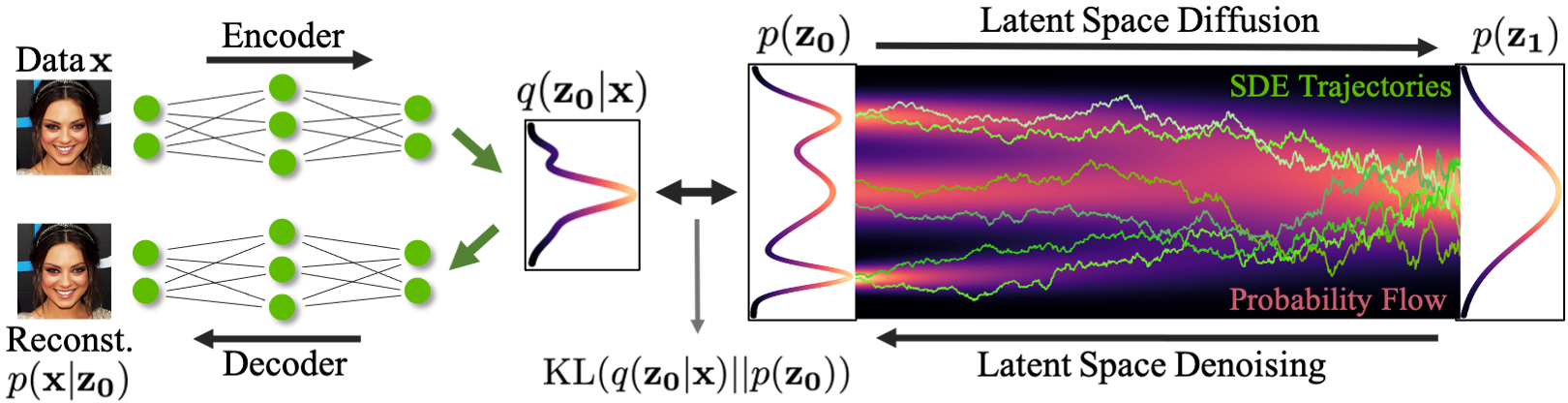
^ Variational Autoencoder (VAE) + Score-based Prior

Main idea: Lift the diffusion models to a latent space which is more friendly to the diffusion process

• Encoder maps the input data to an embedding space
• Denoising diffusion models are applied in the latent space

Advantages:

• The distribution of latent embeddings close to Normal distribution

  • Simpler denoising and faster synthesis

• Augmented latent space

  • More expressivity

• Tailored Autoencoders

  • More expressivity, Application to any data type (e.g. graphs, text, 3d data etc.)

Training objective of LDM: score-matching for cross-entropy

$$\begin{aligned} \mathcal{L}(\mathbf{x}, \boldsymbol{\phi}, \boldsymbol{\theta}, \boldsymbol{\psi}) & =\mathbb{E}_{q_{\boldsymbol{\phi}}\left(\mathbf{z}_0 \mid \mathbf{x}\right)}\left[-\log p_{\boldsymbol{\psi}}\left(\mathbf{x} \mid \mathbf{z}_0\right)\right]+\mathrm{KL}\left(q_{\boldsymbol{\phi}}\left(\mathbf{z}_0 \mid \mathbf{x}\right) \| p_{\boldsymbol{\theta}}\left(\mathbf{z}_0\right)\right) \\ & =\underbrace{\mathbb{E}_{q_{\boldsymbol{\phi}}\left(\mathbf{z}_0 \mid \mathbf{x}\right)}\left[-\log p_{\boldsymbol{\psi}}\left(\mathbf{x} \mid \mathbf{z}_0\right)\right]}_{\text {reconstruction term }}+\underbrace{\mathbb{E}_{q_\phi\left(\mathbf{z}_0 \mid \mathbf{x}\right)}\left[\log q_{\boldsymbol{\phi}}\left(\mathbf{z}_0 \mid \mathbf{x}\right)\right.}_{\text {negative encoder entropy }}]+\underbrace{\mathbb{E}_{q_{\boldsymbol{\phi}}\left(\mathbf{z}_0 \mid \mathbf{x}\right)}\left[-\log p_{\boldsymbol{\theta}}\left(\mathbf{z}_0\right)\right]}_{\text {cross entropy }} \end{aligned}$$

where

• It is optimized by minimizing the variational upper bound negative log likelihood
• the reconstruction term and negative encoder entropy are similar to the training objective of VAE
• the cross entropy term corresponds to the training objective of Diffusion models

Then the objective can be written as

$$C E\left(q\left(\mathbf{z}_0 \mid \mathbf{x}\right) \| p\left(\mathbf{z}_0\right)\right)={\mathbb{E}_{t \sim \mathcal{U}[0,1]}}\left[\frac{g(t)^2}{2} \mathbb{E}_{q\left(\mathbf{z}_t, \mathbf{z}_0 \mid \mathbf{x}\right)}\left[\left\|\nabla_{\mathbf{z}_t} \log q\left(\mathbf{z}_t \mid \mathbf{z}_0\right)-\nabla_{\mathbf{z}_t} \log p\left(\mathbf{z}_t\right)\right\|_2^2\right]\right]+\frac{D}{2} \log \left(2 \pi e \sigma_0^2\right)$$

where

• $\mathbb{E}_{t \sim \mathcal{U}[0,1]}$ is the time sampling
• $\mathbb{E}_q(z_t, z_0|x)$ is the forward diffusion
• $\nabla_{\mathbf{z}_t} \log q\left(\mathbf{z}_t \mid \mathbf{z}_0\right)$ is the diffusion kernel
• $\nabla_{\mathbf{z}_t} \log p(\mathbf{z}_t)$ is the trainable score function
• $\frac{D}{2} \log \left(2 \pi e \sigma_0^2\right)$ is some constant

Conditional Diffusion Models

How to do high-resolution (conditional) generation?

• Reverse process is changed

Reverse Process (taking conditional input $c$):

$$p_\theta(x_{0:T}|c) = p(x_T)\prod^T_{t=1}p_\theta(x_{t-1}|x_t, c)$$

$$p_\theta(x_{t-1}|x_t, c) = \mathcal{N}(x_{t-1}; \mu_\theta(x_t, t, c), \sum_\theta(x_t, t, c))$$

Incorparate conditions into U-Net of the diffusion model

• Scalar conditioning: encode scalar as a vector embedding, simple spatial addition or adaptive group normalization layers
• Image conditioning: channel-wise concatenation of the conditional image
• Text conditioning:
  • single vector embedding: spatial addition or adaptive group norm
  • a sequence of vector embeddings: cross-attention

Classifier Guidance

Diffusion models beat GANs on image synthesis: https://arxiv.org/abs/2105.05233

Using the gradient of a trained classifier as guidance

Main idea:

• For class-conditional modeling of $p(x_t | c)$, train an extra classifier $p(c|x_t)$

  • Mix its gradient with the diffusion/score model during sampling

• Sample with a modified score: $\nabla_{x_t} [\log p(x_t|c) + \omega \log p(c|x_t)]$

• Approximate samples from the distribution $\tilde{p}(x_t|c) \propto p(x_t|c)p(c|x_t)^\omega$

Classifier-Free Guidance

Classifier-Free Diffusion Guidance: https://arxiv.org/abs/2207.12598

Get guidance by Bayes’ rule on conditional diffusion models

Main idea:

• Instead of training an additional classifier, get an “implicit classifier” by jointly training a conditional and unconditional diffusion model
  • $p(x_t|c) \propto p(x_t|c)/p(x_t)$
    • Where $p(x_t|c)$ is the conditional diffusion model, $p(x_t)$ is the unconditional diffusion model
• In practice, $p(x_t|c)$ and $p(x_t)$ by randomly dropping the condition of the diffusion model at certain chance
• The modified score with this implicit classifier included is:
  • $\nabla_{x_t} [\log p(x_t|c) + \omega \log p(c|x_t)] = \nabla_{x_t} [\log p(x_t|c) + \omega (\log p(x_t|c) - \log p(x_t))]$
    • $= \nabla_{x_t} [(1+\omega)\log p(x_t|c) - \omega \log p(x_t)]$

Trade-off for sample quality and sample diversity

• Large guidance weight $\omega$ usually leads to better individual sample quality but less sample diversity

Cascaded generation

Cascaded Diffusion Models for High Fidelity Image Generation: https://cascaded-diffusion.github.io

Main idea:

• Cascaded Diffusion Models (CDM) are pipelines of diffusion models that generate images of increasing resolution.
• CDMs yield high fidelity samples superior to BigGAN-deep and VQ-VAE-2 in terms of both FID score and classification accuracy score on class-conditional ImageNet generation. These results are achieved with pure generative models without any classifier.
• Introduce conditioning augmentation, data augmentation technique that find critical towards achieving high sample fidelity.

Noise conditioning augmentation: Reduce compounding error

Need robust super-resolution model:

• Training conditional on original low-res images from the dataset
• Inference on low-res images generated by the low-res model.

^If there are artifacts in the low-resolution sample will affact the sample quality due to mismatch conditions of two points

To alleviate this problem:

Noise conditioning augmentation

• During training, add varying amounts of Gaussian noise ( or blurring by Gaussian kernel) to the low-res images
• During inference, sweep over the optimal amount of noise added to the low-res images
• BSR-degradation process: applies JPEG compressions noise, camera sensor noise, different image interpolations for downscampling, Gaussian blue kernels and Gaussian noise in a random order to an image.