Rasterization in Computer Graphics

Drawing Triangles

Not everything is triangle but you can always convert them into triangles.

The Graphics Pipeline:

• Input :

  • 3D scene (composed of primitives such as triangles)
  • Camera parameters, lights, etc.

• Output:

  • 2D Image (composed of pixels)

Vertces ===[Pre-vertex operations]===> Transformed vertices ===[Rasterizer]===> Fragments

Fragments ===[Pre-fragment operations]===> Shaded fragments ===[Frame buffer operations]===> Pixels

Rasterization

How to draw the triangle on the signal display using position of triangle vertices?

Let say we have a method called inside(tri,x,y):

def inside(tri, x, y):
  return 1 if (x,y) in tri else 0

But how do we know (x,y) in tri?

How do we sample locations?

for( int x = 0; x < xmax; x++ )
  for( int y = 0; y < ymax; y++ )
    float P_x = x + 0.5;
		float P_y = y + 0.5;
    Image[x][y] = f(P_x, P_y); //Sample location middle point by adding 0.5

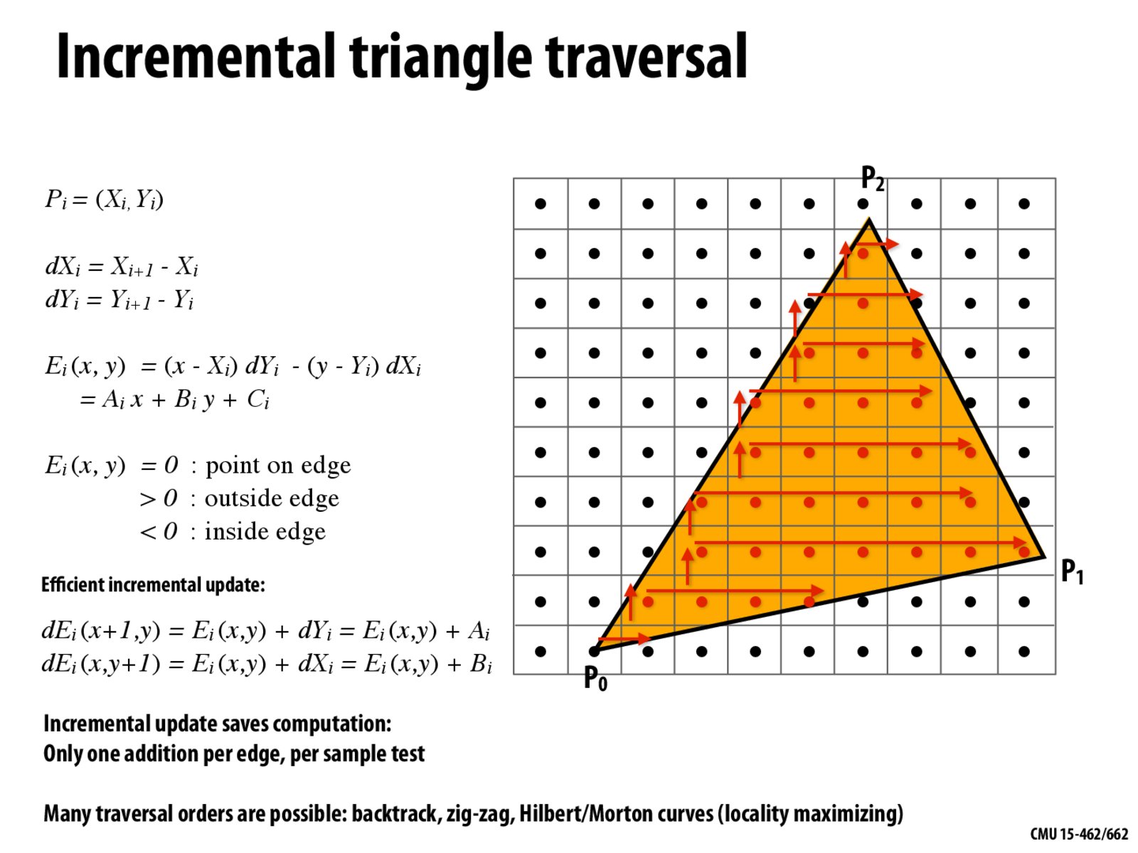
Line Equation Method

• Use Triangle = Intersection of Three Half-Planes rule
  • each line defines two Half-Planes
• $\mathcal{L}(x,y) = Ax + By + C$
  • On line : $\mathcal{L}(x,y) = V \cdot N = 0$
  • Above line : $\mathcal{L}(x,y) = V \cdot N > 0$
  • Below line : $\mathcal{L}(x,y) = V \cdot N < 0$

What is $V \cdot N$ here?

We first derive a Line Tangent Vector $T$ from the line on our plane:

$$T = P_1 - P_0 = (x_1 - x_0, y_1 - y_0)$$

• $T$ is the Line Tangent Vector
• $P_1, P_0$ the two points of a line

Then we get the General Perpendicular Vector in 2D, denote as $N$ which is the perpendicular of $T$.

Since

$$\text{Perpendicular}(x,y) = (-y, x)$$

Then

$$N = \text{Perpendicular}(T) = (-(y_1 - y_0), x_1 - x_0)$$

After that we can define any point connect to $P_0$ as $P$ and have a vector $V$.

$$V = P - P_0 = (x - x_0, y - y_0)$$

Therefore the Line Equation:

$$\mathcal{L}(x,y) = V \cdot N = -(x - x_0)(y_1 - y_0) + (y - y_0)(x_1 - x_0)$$

def line_eq_test(P_0, P_1, P):
  return -(P.x - P_0.x)*(P_1.y - P_0.y) + (P.y - P_0.y)*(P_1.x - P_0.x) 

Then theorically we can :

• Sample point s = (sx, sy) is inside the triangle if it is inside all three lines.

$$\text{inside}(sx, sy) = L_0(sx, sy) > 0\quad \&\& \quad L_1(sx, sy) > 0 \quad\&\&\quad L2 (sx, sy) > 0$$

Note actual implementation of inside(sx, sy) involves $\leq$ checks based on edge rules

struct Triangle {
	float3 positions[3];
	float3 normals[3];
	float2 texcoords[3];
	int idMaterial = 0;
	AABB bbox;
	float3 center;
};
	
bool checkIsInside(const float3 triPosScreen[3], const float P_x, const float P_y) const{
    // Line Equation Method
    // triPosScreen: tri.positions in Screen space (3 vertices from the triangle)
    // P_x: x in Screen
    // P_y: y in Screen
    float L0 = -(P_x - triPosScreen[0].x)*(triPosScreen[1].y - triPosScreen[0].y) + (P_y - triPosScreen[0].y)*(triPosScreen[1].x - triPosScreen[0].x);
    float L1 = -(P_x - triPosScreen[1].x)*(triPosScreen[2].y - triPosScreen[1].y) + (P_y - triPosScreen[1].y)*(triPosScreen[2].x - triPosScreen[1].x);
    float L2 = -(P_x - triPosScreen[2].x)*(triPosScreen[0].y - triPosScreen[2].y) + (P_y - triPosScreen[2].y)*(triPosScreen[0].x - triPosScreen[2].x);

    if ((L0 >= 0) && (L1 >= 0) && (L2 >= 0))
    {return true;}
    else
    {return false;}
}

Think about Edge Cases:

• If a sample point is on the edge of 2 triangles, this sample point belongs to which triangle?

Edge Rules

• When sample point falls on an edge, the sample is classified as within triangle if the edge is a:
  • top edge; or
    • horizontal edge that is above all other edges
  • left edge
    • an edge that is not exactly horizontal and is on the left side of the triangle. (triangle can have one or two left edges)

Another problem of Line Equation Method: How do we find the depth?

How to do Triangle Traversal

Incremental Triangle Traversal

http://15462.courses.cs.cmu.edu/fall2019/lecture/drawingatriangle/slide_068

Tiled Triangle Traversal

http://15462.courses.cs.cmu.edu/fall2019/lecture/drawingatriangle/slide_069

Precomputed hierarchical tiles

Even Modern Approach: Precomputed hierarchical tiles

• We can precompute a set of tiles that are neither “full” nor “empty”.
  • Precompute and store in a 2D table
  • Apply the precomputed tile for those recursively.

Transforms

Linear transform should satisfy the Linear definition:

$$f(x + y) = f(x) + f(y)\\ f(ax) = af(x)$$

However translation itself does not satisfy linear definition.

$$f(x+y) = (x+y) + t \neq f(x) + f(y) = (x+t)+(y+t)\\ f(ax) = ax + t \neq af(x) = a(x+t)$$

Homogeneous coordinate

Homogeneous coordinate refers to represent coordinates in $N$ dimensions with a $(N+1)$-dimension vector.

E.g. Turning a 2D point into Homogeneous coordinate: $(x, y, 1)^T$

$$\mathbf{x} = (x, y) \Rightarrow \mathbf{\bar{x}} = \left[\begin{array}{l} x \\ y \\ 1 \end{array}\right]$$

• $\tilde{\mathbf{x}}=(\tilde{x}, \tilde{y}, \tilde{w})=\tilde{w}(x, y, 1)=\tilde{w} \overline{\mathbf{x}}$
  • Homogeneous coordinates are denoted with a tilde over the vector e.g. $\tilde{x}$
• Why are homogenous coordinates needed in image projection?
  • If you use a homogeneous coordinate system, then you can represent such transformation as linear function.

Alternatively, Turning a 2D vector into Homogeneous coordinate: $(x, y, 0)^T$

Alternatively, for 3D:

• 3D point : $(x, y, z, 1)^T$
• 3D vector: $(x, y, z, 0)^T$

(the last component is usually denoted as $w$). i.e. $(x, y, z, w)^T$

Barycentric Coordinates

2D Linear Interpolation - Way 1

For a given point $x$, measure the distance to each edge; then divide by the height of the triangle:

$$\phi_i(x) = \frac{d_i(x)}{h_i}$$

• $d_i$ is the distance to each edge
• $h_i$ is the height of the triangle

Choosing the 3 sides, then Interpolate by taking linear combination:

$$\hat{f}(x)=f_i \phi_i+f_j \phi_j+f_k \phi_k$$

2D Linear Interpolation - Way 2

We can also get the same three basis functions as a ratio of triangle areas.

$$\phi_i(x)=\frac{\operatorname{area}\left(x, x_j, x_k\right)}{\operatorname{area}\left(x_i, x_j, x_k\right)}$$

• $x$ is the given point
• $x_i, x_j, x_k$ are the vertex point of the triangle

Choosing the 3 sides, then Interpolate by taking linear combination:

$$\hat{f}(x)=f_i \phi_i+f_j \phi_j+f_k \phi_k$$

In implementation, the floating points are not reliable.

2D Linear Interpolation - Way 3 (Best)

http://courses.cms.caltech.edu/cs171/assignments/hw2/hw2-notes/notes-hw2.html

Using this function:

$$f_{i j}(x, y)=\left(y_i-y_j\right) x+\left(x_j-x_i\right) y+x_i y_j-x_j y_i$$

We can express the equations for $\alpha, \beta$, and $\gamma$ in terms of $\mathrm{f}_{\mathrm{ij}}$ in the following manner:

$$\begin{array}{r} \alpha=\frac{f_{b c}\left(x_p, y_p\right)}{f_{b c}\left(x_a, y_a\right)} \\ \beta=\frac{f_{a c}\left(x_p, y_p\right)}{f_{a c}\left(x_b, y_b\right)} \\ \gamma=\frac{f_{a b}\left(x_p, y_p\right)}{f_{a b}\left(x_c, y_c\right)} \end{array}$$

• $a, b, c$ are $x_i, x_j, x_k$
• $p$ is the any point (denoted as $x$ in previous 2 ways)
• $\alpha, \beta, \gamma$ are $\phi_i, \phi_j, \phi_k$ respectively.

float fij(const float2 P, const float2 i, const float2 j) const{
    float f = (i.y - j.y)*P.x + (j.x - i.x)*P.y + i.x*j.y - j.x*i.y;
    return f;
}
float3 computeBarycentricCoordinates(const float2 P, const float2 A, const float2 B, const float2 C) const{
    float alpha = fij(P, B, C) / fij(A, B, C);
    float beta = fij(P, A, C) / fij(B, A, C);
    float gamma = fij(P, A, B) / fij(C, A, B);
    return {alpha, beta, gamma};
}

Barycentric Coordinates - Color Example

By finding $\phi_i(x), \phi_j(x), \phi_k(x)$, we can get the color

$$\operatorname{color}(x)=\operatorname{color}\left(x_i\right) \phi_i+\operatorname{color}\left(x_j\right) \phi_j+\operatorname{color}\left(x_k\right) \phi_k$$

Can be used to interpolate any attribute associated with vertices. (color*, normals, texture coordinates, etc.)

Viewing and Perspective

Consider A Camera Pointing in The World

• Input: e, u & v given in world space coordinates
  • e = eye point (position of camera)
  • u = up vector
  • v = view direction vector
• Output: transform matrix from world space to standard camera space

Camera “Look-At” Transformation

• Given $e, u, v$
  • Assume u and v are orthonormal (same length)
  • Find right vector $r = v \times u$

Then the Derive “Look-at” transform.

The “Look-at” transform is the inverse of Matrix from standard camera to world space (coordinate frame transform to $(e,r,u,-v)$)

$$\left(\begin{array}{cccc} r_x & u_x & -v_x & e_x \\ r_y & u_y & -v_y & e_y \\ r_z & u_z & -v_z & e_z \\ 0 & 0 & 0 & 1 \end{array}\right)^{-1}=\left(\begin{array}{cccc} r_x & r_y & r_z & 0 \\ u_x & u_y & u_z & 0 \\ -v_x & -v_y & -v_z & 0 \\ 0 & 0 & 0 & 1 \end{array}\right) \cdot\left(\begin{array}{cccc} 1 & 0 & 0 & -e_x \\ 0 & 1 & 0 & -e_y \\ 0 & 0 & 1 & -e_z \\ 0 & 0 & 0 & 1 \end{array}\right)$$

// model -> camera matrix
float4x4 lookatMatrix(const float3& _eye, const float3& _center, const float3& _up) const {
	// transformation to the camera coordinate
	float4x4 m;
	const float3 f = normalize(_center - _eye);
	const float3 upp = normalize(_up);
	const float3 s = normalize(cross(f, upp));
	const float3 u = cross(s, f);

	m[0] = { s.x, s.y, s.z, 0.0f };
	m[1] = { u.x, u.y, u.z, 0.0f };
	m[2] = { -f.x, -f.y, -f.z, 0.0f };
	m[3] = { 0.0f, 0.0f, 0.0f, 1.0f };
	m = transpose(m);

	// translation according to the camera location
	const float4x4 t = float4x4{ {1.0f, 0.0f, 0.0f, 0.0f}, {0.0f, 1.0f, 0.0f, 0.0f}, {0.0f, 0.0f, 1.0f, 0.0f}, { -_eye.x, -_eye.y, -_eye.z, 1.0f} };

	m = mul(m, t);
	return m;
}

Perspective Projection

Specifying Perspective Viewing Volume

Parameterized by

• fovy : vertical angular field of view
• aspect ratio : width / height of field of view
• near : depth of near clipping plane
• far : depth of far clipping plane

Derived quantities

• top : near * tan (fovy)
• bottom : –top
• right : top * aspect
• left : –right

Perspective Transform Matrix

$$\mathbf{P}=\left[\begin{array}{cccc} \text { near } & 0 & 0 & 0 \\ \text { right } & \frac{\text { near }}{\text { top }} & 0 & 0 \\ 0 & 0 & -\frac{\text { far+near }}{\text { far-near }} & \frac{-2 \text {far} * \text { fear }}{\text { far-near }} \\ 0 & 0 & -1 & 0 \end{array}\right]$$

// camera -> screen matrix
float4x4 perspectiveMatrix(float fovy, float aspect, float zNear, float zFar) const {
  float4x4 m;
  const float f = 1.0f / (tan(fovy * DegToRad / 2.0f));
  m[0] = { f / aspect, 0.0f, 0.0f, 0.0f };
  m[1] = { 0.0f, f, 0.0f, 0.0f };
  m[2] = { 0.0f, 0.0f, (zFar + zNear) / (zNear - zFar), -1.0f };
  m[3] = { 0.0f, 0.0f, (2.0f * zFar * zNear) / (zNear - zFar), 0.0f };

  return m;
}

Turning Camera Coordinates into Normalized Device Coords

when we say “clip space”, it is equivalent to the normalized device coordinates

// rasterizer
void Rasterize() const {
  // fill in plm by a proper matrix
  const float4x4 pm = perspectiveMatrix(globalFOV, globalAspectRatio, globalDepthMin, globalDepthMax);
  const float4x4 lm = lookatMatrix(globalEye, globalLookat, globalUp);
  const float4x4 plm = mul(pm, lm);
  /*
  plm here means prespective matrix, lookAt matrix (or view matrix) and model matrix. The first two matrices are decided by the camera and the last matrix is decided by each model (here I think model matrix is Identity for the assignment). You can get plm matrix by multiplying the three matrices together and this matrix provides you a convertion from model space to clip space. You need to be careful about the order of the multiplication. 
  */
  FrameBuffer.clear();
  for (int n = 0, n_n = (int)objects.size(); n < n_n; n++) {
    for (int k = 0, k_n = (int)objects[n]->triangles.size(); k < k_n; k++) {
      objects[n]->rasterizeTriangle(objects[n]->triangles[k], plm);
    }
  }
}

• Make the Homogeneous coordinate (x, y, z, w)
• Then multply plm and Homogeneous coordinate
• Then normalize it as (x/w, y/w, z/w, w/w)
• finally map it into screen space

void rasterizeTriangle(const Triangle& tri, const float4x4& plm) const {
      float4 affine_tri;
      for (int i = 0; i < 3; i++) {
          affine_tri = {tri.positions[i].x, tri.positions[i].y, tri.positions[i].z, 1};
          affine_tri = mul(plm, affine_tri);
          affine_tri = {affine_tri.x/affine_tri.w, affine_tri.y/affine_tri.w, affine_tri.z/affine_tri.w, affine_tri.w/affine_tri.w};
          int x = (affine_tri.x + 1.0f) * globalWidth / 2.0;
          int y = (affine_tri.y + 1.0f) * globalHeight / 2.0;
          FrameBuffer.pixel(x, y) = float3(1.0f);
          FrameBuffer.valid(x, y);
      }
}

Helper function for mapping ndc into screen space:

float4 ndc2screen(const float4 homoPos) const{
    //ndc is -1 to 1
    float x = linalg::lerp(0.0f, globalWidth, (homoPos.x + 1.0f) * 0.5f);
    float y = linalg::lerp(0.0f, globalHeight, (homoPos.y + 1.0f) * 0.5f);
    float z = linalg::lerp(globalDepthMin, globalDepthMax, (homoPos.z + 1.0f) * 0.5f);
    float w = homoPos.w;
    float4 screenPos = {x, y, z, w};
    return screenPos;
}

Perspective Correct Interpolation

• Goal: interpolate some attribute ɸ at vertices (not the phi from the barycentric coords)

  • We can interpolate texture coordinate.x , or texture coordinate.y

• Idea: P := ɸ/w interpolates linearly in 2D

Basic recipe:

• Keep the homogeneous coordinate w at each vertex before the division (of course, otherwise w = 1!)
• Evaluate W := 1/w and P := ɸ/w at each vertex
• Interpolate W and P using standard (2D) barycentric coords
• At each pixel, divide interpolated P by interpolated W to get final value
• Depth d = z/w can be interpolated linearly (no division by W is needed since we want depth, not z)

So basically:

• Interpolated w: $w=\frac{\alpha_1}{w_1}+\frac{\alpha_2}{w_2}+\frac{\alpha_3}{w_3}$
• Interpolated p for each diamension: $p=\frac{\alpha_1 \cdot \text { ɸ }_1}{\omega_1}+\frac{\alpha_2 \cdot \text { ɸ }_2}{\omega_2}+\frac{\alpha_3 \cdot \text { ɸ }_3}{w_3}$
• pixel value for each diamension $=$ Interpolated $p /$ Interpolated $w$
• Depth $d=\alpha_1 \cdot \frac{z_1}{w_1}+\alpha_2 \cdot \frac{z_2}{w_2}+\alpha_3 \frac{z_3}{w_3}$
• where $\alpha_1, \alpha_2, \alpha_3$ are $\phi(x_i), \phi(x_j), \phi(x_k)$ from barycentric coords

Depth buffering (Z-buffer)

• Z-buffer uses interpolated depth d = z/w in 2D

• Stores a depth value per pixel

• Overwrites by a pixel closer to the camera

• Depth $d=\alpha_1 \cdot \frac{z_1}{w_1}+\alpha_2 \cdot \frac{z_2}{w_2}+\alpha_3 \frac{z_3}{w_3}$

• where $\alpha_1, \alpha_2, \alpha_3$ are $\phi(x_i), \phi(x_j), \phi(x_k)$ from barycentric coords

Hidden-surface-removal algorithm

Initialize depth buffer to infty 
During rasterization:
  for (each triangle T)
    for (each sample (x,y,depth) in T)
      if (depth < depthbuffer[x,y]) # // closest sample so far
      	framebuffer[x,y] = rgb; # // update colour
        depthbuffer[x,y] = depth; # // update depth
      else
				# // do nothing, this sample is not closest