Quick Review on SVM, Neural Network, CNN and K-means clustering

Support vector machine

• SVM is Supervised learning
• Used For Classification problems
  • Only work on linearly separable data
• Make use of Geometry

SVM is a model-based learning method. After model is built, the training data can be discarded.

• Given data points $X$ in an $n$ dimensional feature space
• SVM separates these data points with an $(n-1)$ dimensional hyperplane.

SVMs aim at solving classification problems by classifing data points with the hyperplane that has the max distance to the nearest data point on each side.

• Decision plane is determined by the perpendicular of the 2 cloest vectors .

Parameter C

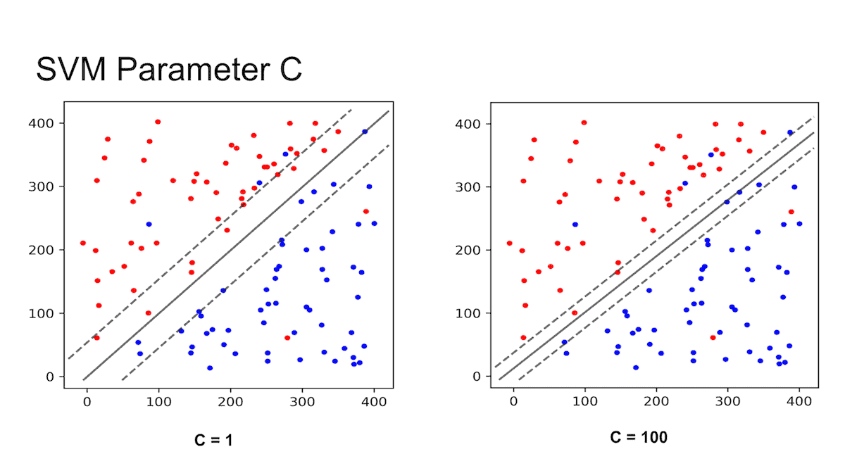
• Lower C value => wider margin
• Higher C value => closer margin

Kernel Functions of SVM

SVM only work on linearly separable data

• Sometimes the data are not linearly separable, we need to process them
• To make data linearly separable, we can use kernel functions

In case the training data $X$ are not linearly separable, we may use a non-linear function $\phi(\mathrm{x})$ to map the data from the input space to a new high-dim space (called feature space $\phi$ ) where data become linearly separable.

• kernel to project input data(features) to a higher dimension
  • Hope that input data is separable in higher dimension
  • some common used kernel function: Polynomial learning machine, Gaussian radial-basis function (RBF)

Summary of SVM

• Decision boundary change significantly if the nearest data points changed
  • since the hyperplane that has the max distance to the nearest data point on each side will be changed.
• The linear SVM is less effective when
  • The data is noisy and contains overlapping points

Neural Networks and Deep Learning

• Neural Network is Supervised learning
• Neural Networks (NN) or Artificial neural networks (ANN) or connectionist systems are computing systems vaguely inspired by the biological neural networks that constitute animal brains.

Model: transforms inputs into outputs, through non-linear information processing

• is a computational model that simulates biological neurons and the way they function in our brain

The general formula is :

$$\text{Output} = Activation(W \cdot X + B)$$

Where $W$ are the weights, $X$ are the inputs, $B$ are the bias, and $Activation$ is the non-linear function called activation function.

A single neuron with no non-linearity can be considered as a linear regression function

A neuron can has single/multiple inputs and single/multiple outputs.

Common Activation functions

ReLU (Rectified Linear Unit)

$$f(x)=\left\{\begin{array}{l} 0 \text { for } x<0 \\ x \text { for } x \geq 0 \end{array}\right.$$

Just max(0,x).

ReLUs enable fast learning and are more resilient to the vanishing gradient problem compared to other functions like the sigmoid.

Leaky ReLU

$$f(x)=\left\{\begin{array}{l} \alpha x \text { for } x<0 \\ x \text { for } x \geq 0 \end{array}\right.$$

where $\alpha$ is a small constant fraction

Like the normal ReLU, but instead of 0, a small constant fraction of x is returned.

Generally we choose a small $\alpha$ value such as 0.01 . Also it stays fixed during traiing.

Gaussian

$$f(x)=e^{-x^{2}}$$

A bell-shaped curve whose maximum value tops out at 1 when x = 0.

Sigmoid

$$f(x)=\frac{e^{x}}{e^{x}+1} = \frac{1}{1+e^{-x}}$$

Sigmoid activation are often only used in the final layer of a neural network. Because the output is continuous and bounded between 0 and 1, sigmoid neurons are a good proxy for output probabilities.

Often represented as $\sigma$.

Softmax

$$f(x_i) = \frac{e^{x_i}}{\sum_k e^{x_k}}$$

where

• $x$ is a set of input values
• $x_i$ is the i-th element in the set of input values
• $k$ is the total number of input values

Outputs multiple values that sum to 1.

Softmax activation are often used in the final layer of a neural network to represent classification probabilities. Because Softmax forces all outputs from a neuron to sum to 1.

A small example to understand softmax calucation easily:

Let $x = \{8,4,2\}$

$\sum_k e^{x_k} = e^8 + e^4 + e^2 = 2980.95799 + 54.59815 + 7.3890561 = 3042.9452$

$f(x_1) = f(8) = \frac{e^8}{e^8 + e^4 + e^2} = \frac{2980.95799}{3042.9452} = 0.979629206 = 0.98$

$f(x_2) = f(4) = \frac{e^4}{e^4 + e^4 + e^2} = \frac{54.59815}{3042.9452} = 0.0179425348 = 0.018$

$f(x_3) = f(2) = \frac{e^2}{e^8 + e^4 + e^2} = \frac{7.3890561}{3042.9452} = 0.00242825802 = 0.002$

Note the summation $\sum_i f(x_i) = 1$

Simple Neural Network Example

Input size = 1

Hidden Layer size = 2

Output layer size = 1

• Feature extraction happens at hidden layers
• This is a fully connected layer (also known as Dense layer), since every neurons are fully connected.
• The fully connected layer is also known as Multilayer perceptron.

Calulating the output with given weights

Lets assume sigmoid activation $(\sigma)$ is use everywhere in this network.

Note the Sigmoid function $f(x) = \frac{1}{1+e^{-x}}$.

$h_1 = \sigma(x_1 \times w_{(x_1,h_1)} + x_2 \times w_{(x_2,h_1)} + b_{h_1}) = \sigma(1\times 1+2\times 0.5 + 0.3) = \sigma(2.3) = \frac{1}{1+e^{-2.3}} = 0.909$

$h_2 = \sigma(x_1 \times w_{(x_1,h_2)} + x_2\times w_{(x_2,h_2)} + b_{h_2}) = \sigma(1\times 0.5 + 2\times 1 + 0.5) = \sigma(3) = \frac{1}{1+e^{-3}} = 0.953$

$o_1 = \sigma(h_1 \times w_{(h_1,o_1)} + h_2 \times w_{(h_2,o_2)} + b_{o_1}) = \sigma(0.909 \times 0.5 + 0.953 \times 0.5 + 0) = \sigma(0.931) = \frac{1}{1+e^{-0.931}} = 0.717$

Calulating the number of parameters in Neural Network

weights and bias are the parameters.

The general formula :

$$\text{No. of Parameters in Input-Hidden} = \text{Input nodes}\times \text{Hidden Nodes } + \text{Hidden Nodes }$$

$$\text{No. of Parameters in Hidden-Output} = \text{Hidden nodes} \times \text{Output nodes } + \text{Output nodes}$$

$$\text{Total No. of Parameters} = \text{No. of Parameters in Input-Hidden} + \text{No. of Parameters in Hidden-Output}$$

Example:

• Input-Hidden: 2x2 (weights) + 2 (bias)= 6
• Hidden-output: 2x1 (weights) + 1 (bias) = 3
• Total parameters = 6+3 = 9

Another example

• Input layer: 8 neurons

• Hidden layer 1: 12 neurons

• Hidden layer 2: 8 neurons

• Output layer: 1 neuron

Find the number of parameters.

No. of Parameters in Input-Hidden1 = 8 x 12 + 12 = 108
No. of Parameters in Hidden1-Hidden2 = 12 x 8 + 8 = 104
No. of Parameters in Hidden2-Output = 8 x 1 + 1 = 9

Total:
108 + 104 + 9 = 221 parameters

Learning is done by Gradient descent to minimize loss.

Gradient descent

• Find minimum point

Update rule:

$$\begin{aligned}w_{i} &=w_{i}-\left(\alpha \times \frac{\partial L}{\partial w_{i}}\right) \\b &=b-\left(\alpha \times \frac{\partial L}{\partial b}\right)\end{aligned}$$

Where $\alpha$ is learning rate and $L$ is the loss function.

Back-propagation is a way where we can calculate the update gradient through partial derivation

• Gradient is found using Back-propagation
  • Back-propagation work backwards: from the output layer -> hidden layer -> input layer
  • We want to differentiate the loss function with respect to the weight (which is unknown).
    • some variable are introduced in between so we can use chain rule to get the gradient

$$\frac{\partial L}{\partial w_{i}}=\frac{\partial L}{\partial \hat{y}} \times \frac{\partial \hat{y}}{\partial z} \times \frac{\partial z}{\partial w_{i}}$$

An Simple Example:

Assume sigmoid $\sigma(z)=\frac{1}{1+e^{-z}}$ is used as activation function here

Assume $L = \sum^N_{i=1}(O_{1i}-y_i)^2$ is used as Loss function here

$$\begin{array}{l}h_{1}=\sigma\left(x_{1} w_{1}+x_{2} w_{2}+b_{1}\right) \\h_{2}=\sigma\left(x_{1} w_{3}+x_{2} w_{4}+b_{2}\right) \\O_{1}=\sigma\left(h_{1} w_{5}+h_{2} w_{6}+b_{3}\right)\end{array}$$

Assume we want to update $w_3$. carry partial differentiation. we should see the $y_{pred}$ term.

$$\frac{\partial L}{\partial w_{3}} = \sum_{i=1}^{N} 2\left(O_{1 i}-y_{i}\right) \frac{\partial O_{1 i}}{\partial w_{3}}$$

$O_{1}=\sigma\left(h_{1} w_{5}+h_{2} w_{6}+b_{3}\right)$, we sub $\left(h_{1} w_{5}+h_{2} w_{6}+b_{3}\right)$ as $t$.

Consider the term $\frac{\partial O_{1 i}}{\partial w_{3}}$

$$\frac{\partial O_{1 i}}{\partial w_{3}} = \frac{\partial \sigma\left(h_{1} w_{5}+h_{2} w_{6}+b_{3}\right)}{\partial w_{3}} = \frac{\partial \sigma(t)}{\partial w_{3}} = \frac{\partial}{\partial w_3}(1+e^{-t})^{-1}$$

Carry partial differentiation again.

$$\frac{\partial \sigma(t)}{\partial w_{3}} = \frac{\partial}{\partial w_3}(1+e^{-t})^{-1} = \frac{-1}{(1+e^{-t})^2}\frac{\partial e^{-t}}{\partial w_3}$$

Consider the term $\frac{\partial e^{-t}}{\partial w_3}$

$$\frac{\partial e^{-t}}{\partial w_3} = -e^{-t}\frac{\partial(t)}{\partial w_3} = -e^{-t}\frac{\partial (h_1w_5 + h_2w_6 + b_3)}{\partial w_3}$$

Carry partial differentiation again. Note we we only have to consider the term related to $w_3$

$h_{2}=\sigma\left(x_{1} w_{3}+x_{2} w_{4}+b_{2}\right)$

Therefore $h_1w_5$ and $b_3$ are treated as constant here.

Consider $\frac{\partial (h_1w_5 + h_2w_6 + b_3)}{\partial w_3}$

$$\frac{\partial (h_1w_5 + h_2w_6 + b_3)}{\partial w_3} = \frac{0+\partial (h_2w_6)+0}{\partial w_3} = w_6\frac{\partial (\sigma\left(x_{1} w_{3}+x_{2} w_{4}+b_{2}\right))}{\partial w_3}$$

Then carry partial differentiation again…

Gradient descent is actually time-consuming because it compute gradient for each training input

• Lots of training input => slow learning

Stochastic gradient descent

In Gradient Descent or Batch Gradient Descent, we use the whole training data per epoch whereas, in Stochastic Gradient Descent, we use only single training example per epoch and Mini-batch Gradient Descent lies in between of these two extremes, in which we can use a mini-batch(small portion) of training data per epoch, thumb rule for selecting the size of mini-batch is in power of 2 like 32, 64, 128 etc.

• speed up calculation
• usually provide a good estimate

Actual process of SGD:

• Divide training data into a number of mini-batch
• Pick out a randomly chosen mini-batch of training inputs -> training
• Pick out another randomly chosen mini-batch and train again
• After exhausting all training inputs it means an epoch of training is complete.
• Start another new training epoch (back to step 2)

Cost function

Mean square error

Mean square error is a commonly used loss function for regression tasks.

$$\text{MSE} = \frac{1}{n} \sum_{i=1}^{n}\left(y_{\text {true }}-y_{p r e d}\right)^{2}$$

• Measures the squared difference between training dataset true label and model predicted label

MSE is not good enough. Because it might encounter slow learning due to initial slope is close to 0

Cross-entropy

Cross-entropy is a commonly used loss function for classification tasks.

$$\text{Cross-entropy} =-\frac{1}{n} \sum_{x}[y \ln a+(1-y) \ln (1-a)]$$

• Measures the difference between the model’s predicted prob distribution and the training dataset’s prob distribution

Binary Cross-entropy of (target, predict)

$$-\sum_n (t \ln p + (1-t) \ln (1-p))$$

Neutral log is used here because it is more convenient when later do differentiation.

• In Binary classification, the label is either 0 or 1

Example: NN prediction: {P(label 0), P(label 1)}

Case1 (Confident): Output from NN: {0.1, 0.9}, true label is 1

Cross entropy of case 1 = $-(0\ln(0.1)+(1-0)\ln(0.9)) = 0.105$

Case2 (Not Confident): Output from NN: {0.4, 0.6}, true label is 1

Cross entropy of case 2 = $-(0\ln(0.4)+(1-0)\ln(0.6)) = 0.511$

Case3 (Wrong Prediction): Output from NN: {0.9, 0.1}, true label is 1

Cross entropy of case 3 = $-(0\ln(0.9)+(1-0)\ln(0.1)) = 2.30$

Small difference: small value, Lage difference: large value

Overfitting and Underfitting

Underfitting

• Lazy model: always predicts a constant value => stable performance, but the model is under-fitting => fail o learn anything about the data, its underlying patterns and relationships
• Symptom: High training error

Overfitting

• Try to fit every data point it encounters => learn the noise as well
• Symptom: Low training error but High testing error or validation error

Solution for overfitting

• Increase the number of training data
• Regularization (sometimes called weight decay)
  • Introduces an extra term in the cost function
  • Reduce the gap between training error and testing error

E.g. Regularization on Cross Entropy function

$$C=-\frac{1}{n} \sum_{x}[y \ln a+(1-y) \ln (1-a)]+\frac{\lambda}{2 n} \sum_{w} w^{2}$$

• Regularization parameter : $\frac{\lambda}{2n}$

Hyper-parameters

Parameters that need to be set before model training (do not have dependency on data)

• Learning rate, regularization parameter, mini- batch size, …

Callbacks

Early stopping

• When cost doesn’t decrease for a number of epochs => save network parameters and stop training

Learning rate scheduler

• When cost doesn’t decrease for a number of epochs => decrease the learning rate (e.g., half it)

Deep Learning

Deep Learning is basically Neural networks with more than 1 fully connected hidden layers.

• Deep learning is a subset of machine learning
• Generally, Deep learning perform better than machine learning when the amount of data is huge.

Deep learning (More hidden layers):

• computationally more complicated than less hidden layers NN
• better generalization capabilities than less hidden layers NN
• Increasing number of hidden layers does not always lead to higher accuracy
• Increasing number of hidden layers could lead to overfitting above certain point.

Deep Convolutional Neural Networks

Convolutional Neural Networks (CNN) are often used in Computer Vision problems.

Classical CNN Consist of two parts:

• Feature extractor (Convolutional layers and Pooling layers)
  • Extract feature from low level to high level
• Trainable classifier (Fully connectly layers)

Some history:

ImageNet challenge winners networks

Convolutional layer

Apart from Fully connected layer (Dense layer) we see from previous section, there is a type of layer called convolutional layer.

• Convolutional layers can extract local features from input data spatially.
• Also use less parameters than Fully connected layers.

Convolution in Convolutional layer

• Size of the block is called kernel/filter size
• Extract local features

The default convolution operation in Convolutional layer is not the same way we do in digital image processing. The output size will not be the same as input since we won’t extend the boundary.

A quick example (a convolutional layer with 1 filter) :

Pooling layer

• Pooling layer is introduced to reduces the dimensionality of feature.
  • Often put right after Convolutional layer
  • Pooling can be average pooling or maximum pooling

A quick example (a max pooling layer with 2x2 filters and 2 strides) :

• Stride = 2 means the it slide 2 blocks each time.

Dropout layer

This layer is used to fight against overfitting.

• Randomly (temporarily) deleting some of the neurons of the network in the training process
• Usually put 1 after pooling layer, or before FC layer
• Dropout almost doubbles the time to converge in training.

K-means clustering

• K-means clustering is Unsupervised learning
  • Since clustering itself is a unsupervised learning method
    • assignment of objects into groups (called clusters) so that objects from the same cluster are more similar to each other than objects from different clusters
  • partitions x into k clusters
• Features cannot be categorical
  • It is simply not possible to use the k-means clustering over categorical data because you need a distance between elements and that is not clear with categorical data as it is with the numerical part of your data.
• Feature scaling is needed
  • Feature scaling ensures that all the features get same weight in the clustering
• Used For Classification problems
• Make use of Geometry

Algorithm of K-means clustering

K-means clustering: how it works

1. Choose the number of clusters (K), and input a set of points (X)
2. Specify the cluster seeds (place centroid at random location for each cluster)
3. For each point, find the nearest centroid by comparing the euclidean distance. Assign that point to the cluster that has nearest centroid.
4. For each clusters, Assign a centroid which is equal to the mean of all points in that cluster.
5. Repeat 3 and 4 until we can no longer reassign points (convergence)

Euclidean distance formula:

$$E(x, y)=\sqrt{\sum_{i=0}^{n}\left(x_{i}-y_{i}\right)^{2}}$$

Example of new clusters’ centers after one iteration

Use the $k$ -means algorithm and Euclidean distance to cluster the following 8 examples into 3 clusters.

Let $\mathrm{A}_{i}$ denotes the $i$ -th example and contains two features written as $\left(f_{1}, f_{2}\right)$.
$\mathrm{A}_{1}=(2,10), \mathrm{A}_{2}=(2,5), \mathrm{A}_{3}=(8,4), \mathrm{A}_{4}=(5,8), \mathrm{A}_{5}=(7,5), \mathrm{A}_{6}=(6,4), \mathrm{A}_{7}=(1,2), \mathrm{A}_{8}=(4,9)$

Suppose that the initial centers are $\mathrm{A}_{1}, \mathrm{~A}_{4}$ and $\mathrm{A}_{7}$. Find out the new clusters’ centers after one iteration.

	Distance to A1	Distance to A4	Distance to A7
A1	0	3.606	8.062
A2	5	4.242	3.162
A3	8.485	5	7.280
A4	3.606	0	7.211
A5	7.071	3.606	6.708
A6	7.021	4.123	5.385
A7	8.062	7.211	0
A8	2.236	1.414	7.616

After one iteration:

Cluster 1: A1
New Cluster 1 center: (A1)/1 = (2,10)

Cluster 2: A3, A4, A5, A6, A8
New Cluster 2 center: (A3+A4+A5+A6+A8)/5 = (6,6)

Cluster 3: A2, A7
New Cluster 3 center: (A2+A7)/2 = (1.5, 3.5)

Example of assigning new centroid

With the use of K-means clustering, 7 observations are clustered into 3 groups. After the first iteration, C1, C2 and C3 have the following observations

• C1: {(2,2), (4,4), (6,6)}
• C2: {(0,4), (4,0)}
• C3: {(5,5), (9,9)}

What will be the cluster centroids for C1, C2, C3?

For each clusters, Assign a centroid which is equal to the mean of all points in that cluster.

new centroid of C1: $\frac{(2,2) + (4,4) + (6,6)}{3} = (4,4)$

new centroid of C2: $\frac{(0,4)+(4,0)}{2} = (2,2)$

new centroid of C3: $\frac{(5,5)+(9,9)}{2} = (7,7)$

The 3 possible termination conditions in K-means clustering

• Centroids do not change between successive iterations. (This also ensures that the algorithm has converged to minima)
• For a fixed number of iterations: limits the runtime of the clustering algorithm, but in some cases the quality of the clustering will be poor because of an insufficient number of iterations
• Assignment of observations to clusters does not change between iterations: Except for cases with a bad local minimum, this produces a good clustering, but runtimes maybe unacceptably long

Silhouette Analysis

Help us to decide the K value hyperparameter.

The silhouette coefficient is a measure of how similar an object is to its own cluster compared to other clusters. Number of clusters for which silhouette coefficient is highest represents the best choice of the number of clusters

• The silhouette coefficient is a value between -1 and 1.
  • Higher value(around 1) means an object is to its own cluster compared to other clusters is highly similar (good result)
  • Lower value(-1 to 0) means bad result and the separation is not very good
• We need to calucate 2 distances formula in order to get a silhouette for a sample.
  • for N samples, we need to calucate N times and add up all the silhouette and divide by N.

Silhouette for 1 sample

The formula for $s(i)$ silhouette score (considering only 1 sample):

$$s(i)=\frac{b(i)-a(i)}{\max \{a(i), b(i)\}}=\left\{\begin{array}{ll} 1-\frac{a(i)}{b(i)} & \text { if } a(i)<b(i) \\ 0 & \text { if } a(i)=b(i) \\ \frac{b(i)}{a(i)}-1 & \text { if } a(i)>b(i) \end{array}\right.$$

where

• $a(i)$ Cohesion : mean distance between data point $i$ and all data points in the same cluster
  • smaller $a(i)$ the better

$$a(i)=\frac{1}{\left|C_{i}\right|-1} \sum_{j \in C_{i}, i \neq j} d(i, j)$$

• $b(i)$ Separation : smallest mean distance of data point $i$ to points in other clusters

$$b(i)=\min _{k \neq i} \frac{1}{\left|C_{k}\right|} \sum_{j \in C_{k}} d(i, j)$$

If the silhouette score is close to 1, it means a(i) is small and b(i) is large.

Silhouette coefficient for all sample

The Silhouette Coefficient is calculated using the mean intra-cluster distance (a) and the mean nearest-cluster distance (b) for each sample. The Silhouette Coefficient for a sample is (b - a) / max(a, b).

The formula for silhouette coefficient (considering all samples)

$$SC = \frac{1}{N}\sum^N_{o=0} s(i)$$

Summary of K-means clustering

Advantages of K-means

• Simple to understand
• Fast to cluster
• Widely available
• Easy to implement
• Always yields a result

Disadvantages of K-means

• Sensitive to initial centroid locations
  • Different initialization may cause different result
  • For two runs of K-means clustering, we might or might not obtain the same clustering result.
• Sensitive to outliers
• Produces spherical solutions
• Need to determine to use Standardization or not