Logistic Regression in Python
Logistic Regression Assumption
We should consider them before performing Logistic regression analysis.
- No endogeneity of regressor
- Normality and homoscedasticity
- No autocorrelation
- No multicollinearity
We should not violate the assumptions.
If a regression assumption is violated, performing regression analysis will yeild an incorrect result.
Logistic Regression
On real world problems often require more sophisticated non-linear models.
on-linear models can be :
- Quadratic
- Exponential
- Logistic
Logistic Regression Model
A logistic regression implies that the possible outcomes are not numerical but rather categorical.
E.g. We can use logistic regression to predict Yes / No (Binary Prediction)

- Logistic regression predicts the probability of an event occurring.
- Input => Probability
Logistic Regression Equations
Logistic Regression Equation
Logit Regression Equation
Odds and Binary Predictors
Note: Odds =
In simplifier explaination,
= coef_of_const + coef_of_x1
Note :
Difference of unit of :
= coef_of_x1
Then
e^{coef_of_x1(x1_2 - x1_1)}
When x1 increases by , the odds of y increases by ().
The General Rule:
The change in the odds equals the exponential of the coefficient.
Example of Binary Predictors:
x1 will be only 1 or 0.
= coef_of_x1 = coef_of_x1
By taking exponent you can find the difference of and using numpy.
1 | np.exp(coef_of_x1) |
Then
= np.exp(coef_of_x1)
You can say:
Given the same x1, has np.exp(coef_of_x1) times higher oddeds to get .
Logistic Regression In Python (with StatsModels)
Import the relevant libraries
1 | import pandas as pd |
Load the Data
Just like the same old ways
1 | raw_data = pd.read_csv('xxxyyy.csv') |
Making Dummy variables by mapping all the entries
1 | # We make sure to create a copy of the data before we start altering it. Note that we don't change the original data we loaded. |
Declare the dependent and independent variables
1 | y = data['y'] |
Run the Regression
Just like before, we need to add constant
1 | x = sm.add_constant(x1) |
New Terms in Logistic Regression summary
- MLE (Maximum likelihood estimation)
- The bigger the likelihood function, the higher probability that our model is correct
- Log-Likelihood
- Value of the Log-Likelihood is usually negative
- bigger Log-Likelihood is better
- LL-Null (Log-Likelihood-null)
- the log-likelihood of a model which has no independent variables
- you may want to compare the log likelihood of your model with the LL-Null to see if your model has any explanatory power.
- Pseudo R-squared: McFadden’s R-squared
- A good pseudo r-squared is somewhere between 0.2 and 0.4.
- this measure is mostly useful for comparing variations of the same model.
- Different models will have completely different an incomparable pseudo r-squares.
- P-values
- Check if the model is significant and the variable is significant.
Accuracy
sm.LogitResults.predict() returns the values predicted by our model.
1 | #apply formatting |
Output will show the . I need to round the values to 0 or 1.
Now we show the actual values.
1 | np.array(data['y']) |
- If 80% of the predicted values coincide with the actual values, we say the model has 80% accuracy.
We dont need to compare the tables by ourselfs, just code it into Confusion Matrix.
sm.LogitResults.pred_table()
1 | results_log.pred_table() |
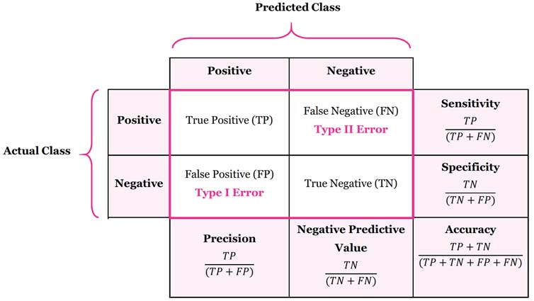
cm_df (Confusion Matrix DataFrame) may look like this:

In this table:
In 159 cases the model did the job well
- For 69 observations the model predicted 0 and the true value was 0 (True Positive)
- For 90 observations the model predicted 1 and the true value was 1 (True Negative)
In 9 cases the model got confused
- For 4 observations the model predicted 0 and the true value was 1 (Type I Error)
- For 5 observations the model predicted 1 and the true value was 0 (Type II Error)
Overall the model made an accurate prediction in 159 out of 168 cases = 94.6% accuracy
1 | # Find the accuracy |
How to check the matrix
Test the model using new data
Use our model to make predictions based on the test data
Load the test dataset
1 | # Load the test dataset |
1 | # Map the test data as you did with the train data |
Remember:
our test data shape should look the same as the input data on which the regression was trained.
order is very important because the coefficients of the regression will expect it.
1 | # Get the actual values (true values ; targets) |
Now test_data will look exactly as x.
Now Create a confusion matrix and calculate the accuracy again.
We write our Confusion Matrix function.
Confusion Matrix shows how confused our model is
1 | def confusion_matrix(data,actual_values,model): |
Usage
1 | # Create a confusion matrix with the test data |
Almost always the training accuracy is higher than the test accuracy. (Overfitting)
Lastly change it into DataFrame.
1 | cm_df = pd.DataFrame(cm[0]) |
- Missclassification rate = 1 - accuracy
Reference
The Data Science Course 2020: Complete Data Science Bootcamp