Probability and Statistics in Data Science
Probability for Data Science
What is Probability?
Probability is the likelihood of an event occurring. This event can be pretty much anything – getting heads, rolling a 4. We measure probability with numeric values between 0 and 1, because we like to compare the relative likelihood of events. Observe the general probability formula.
Probability = quantifying how likely each event is on it’s own
Where X means event, P(x) means probability.
Example: rolling a dice to get value 3, the probability = 1/6.
If Two Events are independent:
Expected Values
- Trial – Observing an event occur and recording the outcome
- Experiment – A collection of one or multiple trials
- Experimental Probability – The probability we assign an event, based on an experiment we conduct
- It is different to theoretical (true) probabilities!
- Expected value – the specific outcome we expect to occur when we run an experiment many times
The expected value can be numerical, Boolean, categorical or other, depending on the type of the event we are interested in.
Expected value – the specific outcome we expect to occur when we run an experiment many times
For instance, the expected value of the trial would be the more likely of the two outcomes, whereas the expected value of the experiment will be the number of time we expect to get either heads or tails after the 20 trials.
We can use expected values to make predictions about the future based on past data
Expected value for categorical variables
Expected value for numeric variables
Probability Frequency Distribution
A collection of the probabilities for each possible outcome of an event.
We need the probability frequency distribution to try and predict future events when the expected value is unattainable.
usually the highest bars in the graph will form the expected value.
Frequency
Frequency is the number of times a given value or outcome appears in the sample space.
Complements
A’ = Not A
is same as
Factorials
Factorials express the product of all integers from 1 to n and we denote them with the “!” symbol.
Key Points
Let n > 0, k > 0 and n > k.
Variations
Variations represent the number of different possible ways we can pick and arrange a number of elements of a given set.
###Variations without repetition
- is the Variations without repetition
- is the number of different elements available
- is the number of elements we are arranging.
Formula Explained:
- We have n-many options for the first element.
- We only have (n-1)-many options for the second element because we cannot repeat the value for we chose to start with.
- We have less options left for each additional element.
###Variations with repetition
- is the Variations with repetition
- is the number of different elements available
- is the number of elements we are arranging.
Formula Explained:
- We have n-many options for the first element.
- We still have n-many options for the second element because repetition is allowed.
- We have n-many options for each of the p- many elements.
Permutations
Permutations represent the number of different possible ways we can arrange a number of elements.
Characteristics of Permutations
- Arranging all elements within the sample space
- No repetition
Combinations
Combinations represent the number of different possible ways we can pick a number of elements.
Characteristics of Combinations
- Takes into account double-counting.
- e.g. Selecting Johny, Kate and Marie is the same as selecting Marie, Kate and Johny
- All the different permutations of a single combination are different variations
- Combinations are symmetric
- e.g. , since selecting p elements is the same as omitting n-p elements
- Apply symmetry to avoid calculating factorials of large numbers (simplify calculations)
Note:
Combinations with separate sample spaces
Combinations represent the number of different possible ways we can pick a number of elements.
Where C is the combinations, is the size of the first sample space, is the size of last sample space.
Characteristics of Combinations with separate sample spaces:
- The option we choose for any element does not affect the number of options for the other elements.
- The order in which we pick the individual elements is arbitrary.
- We need to know the size of the sample space for each individual element.
Combinations with Repetition
Combinations represent the number of different possible ways we can pick a number of elements. In special cases we can have repetition in combinations and for those we use a different formula.
- is the Combinations with repetition
- is the total number of elements in the sample space
- is the number of elements we need to select
Transform combinations with repetition to combinations without repetition
Bayesian Notation
A set is a collection of elements, which hold certain values. Additionally, every event has a set of outcomes that satisfy it.
There always exist a set of outcomes that satisfy a given event.
The null-set (or empty set), denoted , is an set which contain no values.

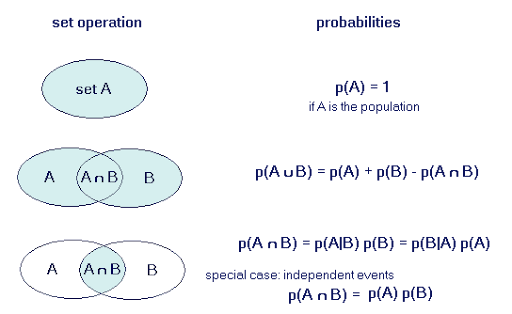
Intersection, Union and Matually Exclusive Sets
Let me quickly go through this.
Intersection
= and
Union
= or
Note : =
Matually Exclusive Sets
If , then the two sets are mutually exclusive.
Independent and Dependent Events
If the likelihood of event A occurring (P(A)) is affected event B occurring, then we say that A and B are dependent events. Alternatively, if it isn’t – the two events are independent.
We express the probability of event A occurring, given event B has occurred the following way:
We call this the conditional probability.
Independent Case
still equals to .
Since the outcome of A does not depend on the outcome of B.
Dependent Case
As the outcome of A depends on the outcome of B,
is not equal to .
Conditional Probability
For any two events A and B, such that the likelihood of B occurring is greater than 0 (𝑃(𝐵) > 0), the conditional probability formula states the following.
Note: does not equal to
Additive Law
The additive law calculates the probability of the union based on the probability of the individual sets it accounts for.
This holds true for any events A and B.
The Multiplication Rule
The multiplication rule calculates the probability of the intersection based on the conditional probability.
Bayes’ Law / Bayes’ Theorem
Bayes’ Law / Bayes’ Theorem helps us understand the relationship between two events by computing the different conditional probabilities.
Fact: Bayes’ Law is often used in medical or business analysis to determine which of two symptoms affects the other one more.
Distributions
A distribution shows the possible values a random variable can take and how frequently they occur.
A distribution is a function that shows the possible values for a variable and how often they occur.
mean = average value
variance = how spread out the data is


Types of Distributions
Certain distributions share characteristics, so we separate them into types.
The well-defined types of distributions we often deal with have elegant statistics.
We distinguish between two big types of distributions based on the type of the possible values for the variable - discrete and continuous.
Discrete
- Have a finite number of outcomes.
- Use formulas we already talked about.
- Can add up individual values to determine probability of an interval.
- Can be expressed with a table, graph or a piece-wise function.
- Expected Values might be unattainable.
- Graph consists of bars lined up one after the other.
Continuous
- Have infinitely many consecutive possible values.
- Use new formulas for attaining the probability of specific values and intervals.
- Cannot add up the individual values that make up an interval because there are infinitely many of them.
- Can be expressed with a graph or a continuous function.
- Graph consists of a smooth curve.
Notation
Discrete Distributions
Discrete Distributions have finitely many different possible outcomes.
Entire probability distribution can be expressed with a table, a graph or a formula
The graph is called Probability density function (PDF).
- CDF represents the sum of all the PDF values up to that point.
They possess several key characteristics which separate them from continuous ones.
Examples:
- Discrete Uniform Distribution
- Bernoulli Distribution
- Binomial Distribution
- Poisson Distribution
All outcomes are equally likely -> Equiprobable
Discrete Uniform Distribution
A distribution where all the outcomes are equally likely is called a Uniform Distribution.
All outcomes are equally likely -> Equiprobable
Both the mean and the variance are uninterpretable
No predictive power
Notation:
~
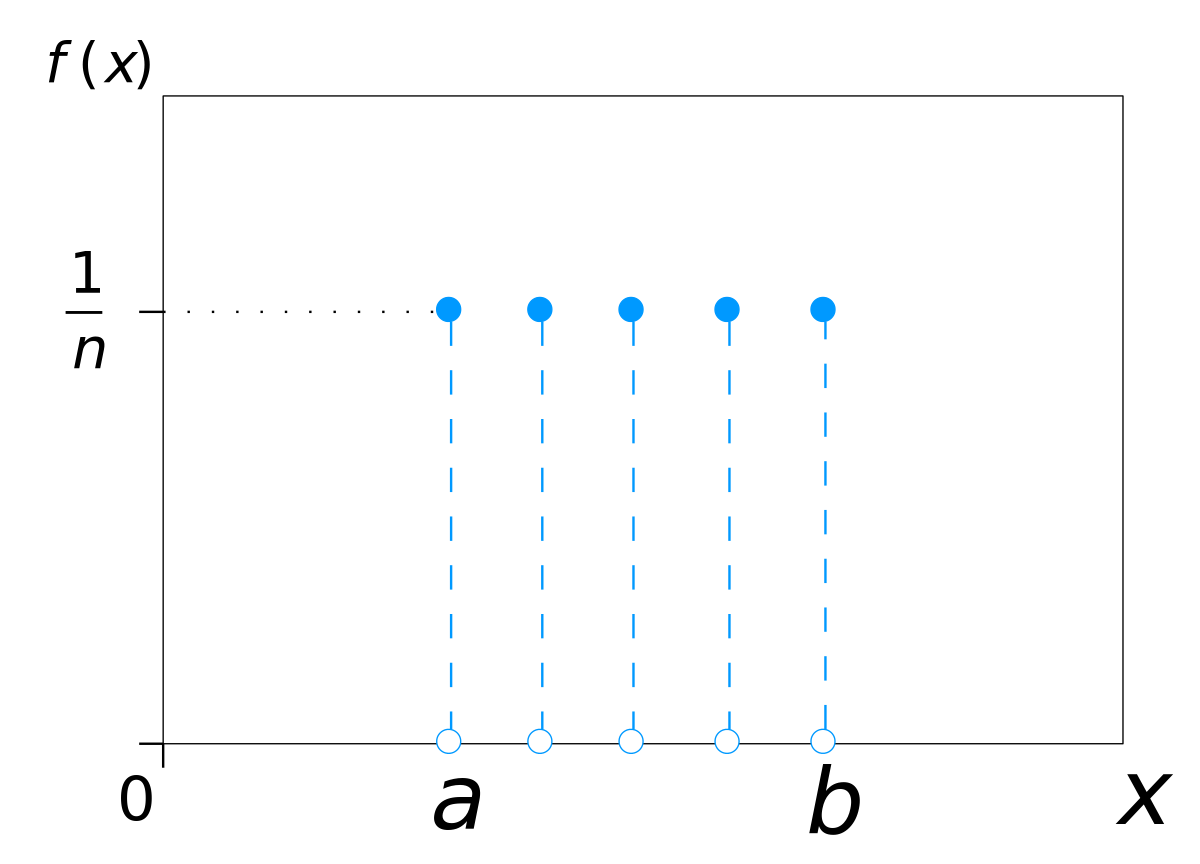
Key Characteristics:
- All outcomes are equally likely.
- All the bars on the graph are equally tall.
- The expected value and variance have no predictive power
Example and uses:
- Outcomes of rolling a single die.
- Often used in shuffling algorithms due to its fairness.
Bernoulli Distribution
A distribution consisting of 1 single trial and only 2 possible outcomes – success or failure is called a Bernoulli Distribution.
Any event with only 2 outcomes can be transformed into a Bernoulli event
Notation:
~
Conventionally we will assign of 1 to the event with the probability =
Assign of 0 to the event with the probability =
Key Characteristics:
- One trial.
- Two possible outcomes.
-
- E(Bernoulli event) = which outcome we expect for a single trial
Example and uses:
- Guessing a single True/False question.
- Often used in when trying to determine what we expect to get out a single trial of an experiment.
Binomial Distribution
A sequence of identical Bernoulli events is called Binomial and follows a Binomial Distribution.
Carrying out a experiment and only two possible outcomes several times in a row
Notation:
~
Where is the number of trials and is the probability of success in each individual trial


Key Characteristics:
- Measures the frequency of occurrence of one of the possible outcomes over the n trials
-
- E(Binomial Event) = the number of times we expect to get a specific outcome
Example and uses:
- Determining how many times we expect to get a heads if we flip a coin 10 times
- Often used when trying to predict how likely an event is to occur over a series of trials
Poisson Distribution
When we want to know the likelihood of a certain event occurring over a given interval of time or distance we use a Poisson Distribution.
Notation:
~
where is mean number of the occurence in the interval.
Key Characteristics:
- Measures the frequency over an interval of time or distance. (Only non-negative values.)
Example and uses:
- Used to determine how likely a specific outcome is, knowing how often the event usually occurs.
- Often incorporated in marketing analysis to determine whether above average visits are out of the ordinary or not.
Continuous Distributions
If the possible values a random variable can take are a sequence of infinitely many consecutive values, we are dealing with a continuous distribution.
The probability distribution would be a curve graph, called Probability distribution curve (PDC).
Examples:
- Normal Distribution
- Chi-Squared Distribution
- Exponential Distribution
- Logistic Distribution
Normal Distribution
Also known as Gaussian Distribution, Bell Curve
A Normal Distribution represents a distribution that most natural events follow.
Notation:
~
Where is mean and is variance.

Note
68% of all outcomes fall within 1 standard deviation away from the mean
95% of all outcomes fall within 2 standard deviation away from the mean
99.7% of all outcomes fall within 3 standard deviation away from the mean

Note:
Dispersion of the distribution depends on Standard Deviation .
a lower standard deviation result in a lower dispersion (denser in the middle) and thinner tail.
a higher standard deviation will cause the graph to flatten out with less points in the middle and more to the end (fatter tail).
Key Characteristics:
- Its graph is bell-shaped curve, symmetric and has thin tails
- 68% of all its values should fall in the interval:
- mean = median = mode
- no skew
Example and uses:
- Often observed in the size of animals in the wilderness
- Could be standardized to use the Z-table
Standard Normal Distribution
To standardize any normal distribution we need to transform it so that the expected value is 0 and the variance and standard deviation are 1.
We move the graph to the left or right until the mean = 0.
Then divide the whole graph with to get standard deviation = 1.
Importance of the Standard Normal Distribution:
- The new variable (Z-score), represents how many standard deviations away from the mean, each corresponding value is.
- We can transform any Normal Distribution into a Standard Normal Distribution using the transformation shown above.
- Convenient to use because of a table of known values for its CDF, called the Z-score table, or simply the Z-table.
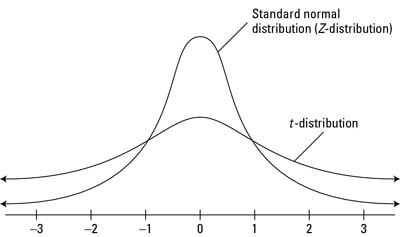
Students’ T Distribution
A small sample size approximation of a Normal Distribution
Student’s-T accommodates extreme values significantly better
Students’ T distribution compares to Normal Ditstribution
- curves having fatter tails
- larger number of values located far away from the mean
Notation
~
where is degrees of freedom.
Key characteristics:
- A small sample size approximation of a Normal Distribution
- Its graph is bell-shaped curve, symmetric, but has fat tails
- Accounts for extreme values better than the Normal Distribution
Example and uses:
- Often used in analysis when examining a small sample of data that usually follows a Normal Distribution. (Not sufficient data and with unknown population variance)
- Hypothesis testing with limited data
- CDF table (t-table)
We can obtain the student’s T distribution for a variable with a Normally distributed population using the formula:
Chi-Squared Distribution
Only consists of non-negative values. Its graph is Asymmetric and skewed to the right.
Used in Hypothesis Testing to help determine goodness of fit
Notation
~
where is degrees of freedom.
Key Characteristics:
- Its graph is asymmetric and skewed to the right.
- Used in Hypothesis Testing
- The Chi-Squared distribution is the square of the t-distribution.
Example and uses:
- Often used to test goodness of fit
- Contains a table of known values for its CDF called the -table. The only difference is the table shows what part of the table
Exponential Distribution
The Exponential Distribution is usually observed in events which significantly change early on.
e.g. Online news articles generate hits
Notation:
~
where is the rate parameter.
This determines how fast the CDF/PDF curve reaches the point of plateauing and how spread out the graph is.
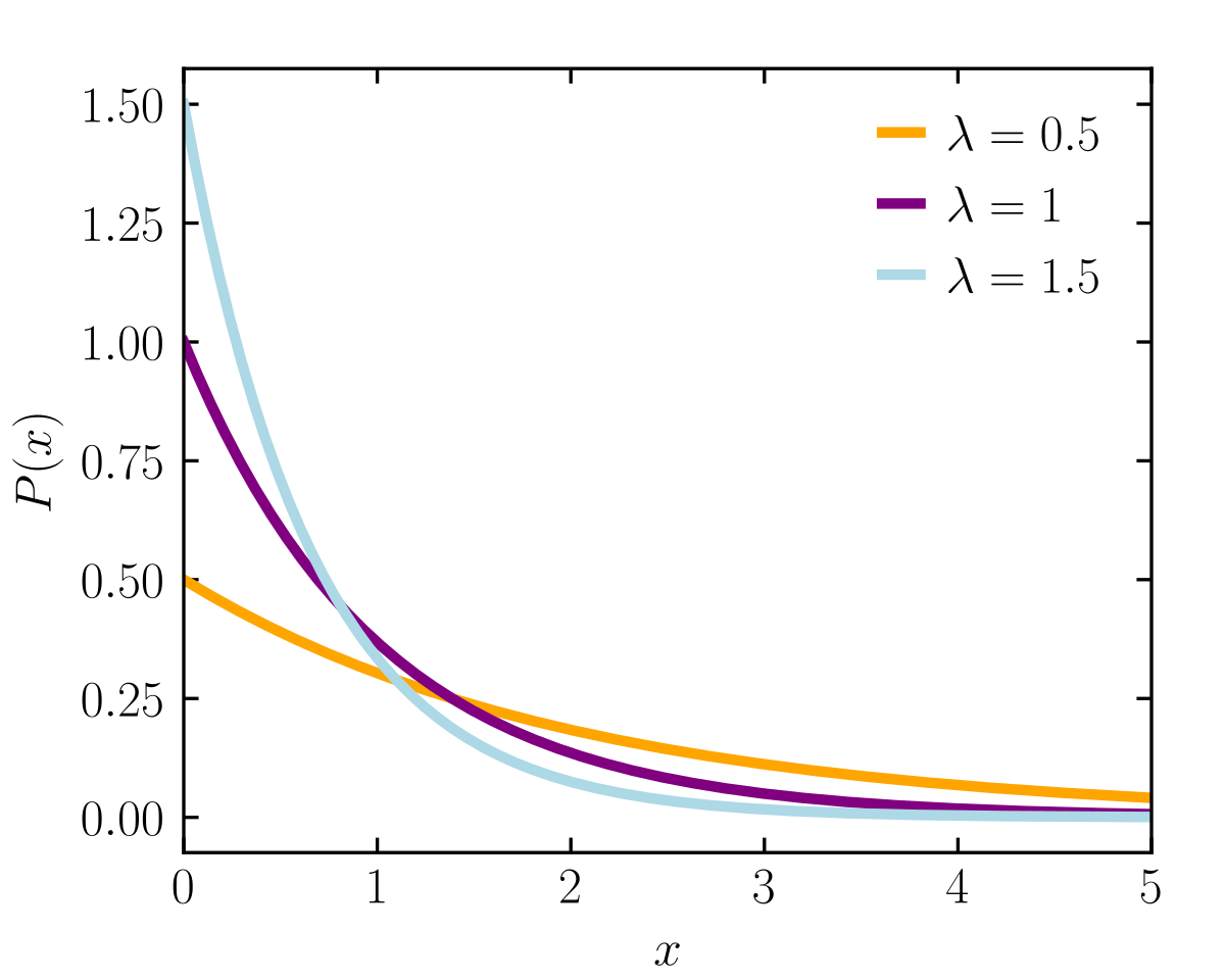
Key Characteristics:
- Both the PDF and the CDF plateau after a certain point.
- We often use the natural logarithm to transform the values of such distributions since we do not have a table of known values like the Normal or Chi- Squared.
- Apply to get normal distribution.
Example and uses:
- Often used with dynamically changing variables, like online website traffic or radioactive decay.
Logistic Distribution
The Continuous Logistic Distribution is observed when trying to determine how continuous variable inputs can affect the probability of a binary outcome.
Useful in forecasting (prediction)
Useful for determing a cut-off point for a successful outcome.
Notation:
~
where is the location and is the scale parameter.
Key Characteristics:
- The CDF picks up when we reach values near the mean.
- The smaller the scale parameter, the quicker it reaches values close to 1.
Example and uses:
- Often used in sports to anticipate how a player’s or team’s performance can determine the outcome of the match.
- Forcasting competitive sports
Statistics
First Step
You need to determine whether the data you are dealing with is a population or a sample.
Population
Collection of all items of interest
Denoted as
The number we’ve obtained when using a population are called Parameters.
Populations are hard to define and hard to observe in real life.
Sample
A subset of the population
Denoted as
The number we’ve obtained when using a sample are called Statistics.
A sample is much easier to gather.
- Less time consuming
- Less costly (cheaper)
Sample
Testicle tests are usually based on sample data
samples are key to accuracy testicle insights.
A sample must be both random and representative for an insight to be precise.
Randomness
a random sample is collected when each member of the sample is chosen from the population strictly by chance.
Representativeness
A representative sample is a subset of the population that accurately reflects the members of the entire population.
Types of Data
Categorical
Categorical data describes categories or groups.
E.g. Car brands, Yes No Questions
Numerical
Numerical data represents numbers.
it is further divided into two subsets - discrete and continuous
Discrete
- Can be counted in finite matter
E.g. Number of objects (Only take integer value)
Continuous
- Infinite and impossible to count
- Just Approximation
E.g. Weight, Distance (All of these can vary by infinitely smaller amounts)
Levels of Measurement
Qualitative Variables
Nominal Variables
- Not numbers and cannot be ordered
E.g. Four Seasons (winter, spring, summer, autumn)
Ordinal Variables
- Followed by order
E.g. Rating your meal (from very bad, bad, neutral, good, very good)
Quantitative Variables
Interval Variables
- Number
- Does not have a true 0
E.g. Temperature (Celsuis and Fahrenheit)
Ratio Variables
- Number
- Has a true 0 point
E.g. Length, Weight
Graphs and Tables
In data science, there are many graphs and tables that represent categorical variables.
Frequency distribution tables (categorical)
Note Frequency distribution tables for numerical variables are different than the ones for categorical.
In Excel
In Excel, we can either hard code the frequencies or count them with a count function. This will come up later on.
Total formula: =SUM()
Bar charts
Called Clustered Column Charts in Excel.
In Excel
Bar charts are also called clustered column charts in Excel.
Choose your data, Insert -> Charts -> Clustered column or Bar chart.
Pie charts
Keyword: Market share
In Excel
Pie charts are created in the following way:
Choose your data, Insert -> Charts -> Pie chart
Pareto Diagrams
Basically a Bar chart shown in descending order of frequency, and a separate curve shows the cumulative frequency.

In Excel
- Order the data in your frequency distribution table in descending order.
- Create a bar chart.
- Add a column in your frequency distribution table that measures the cumulative frequency
- Select the plot area of the chart in Excel and Right click.
- Choose Select series
- Click Add
- Series name doesn’t matter. You can put ‘Line’
- For Series values choose the cells that refer to the cumulative frequency
- Click OK. You should see two side-by-side bars.
- Select the plot area of the chart and Right click.
- Choose Change Chart Type.
- Select Combo.
- Choose the type of representation from the dropdown list. Your initial categories should be ‘Clustered Column.’ Change the second series, that you called ‘Line’, to ‘Line’.
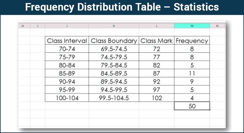
Frequency distribution tables (Numerical)
Frequency distribution tables for numerical variables are different than the ones for categorical. Usually, they are divided into intervals of equal (or unequal) length. The tables show the interval, the absolute frequency and sometimes it is useful to also include the relative (and cumulative) frequencies.
The interval width is calculated using the following formula:
In Excel
-
Decide on the number of intervals you would like to use.
-
Find the interval width (using a the formula above).
-
Start your 1st interval at the lowest value in your dataset.
-
Finish your 1st interval at the lowest value + the interval width. ( = start_interval_cell + interval_width_cell )
-
Start your 2nd interval where the 1st stops (that’s a formula as well - just make the starting cell of interval 2 = the ending of interval 1)
-
Continue in this way until you have created the desired number of intervals.
-
Count the absolute frequencies using the following COUNTIF formula: =COUNTIF(dataset_range,“>=“&interval start) -COUNTIF(dataset_range,”>“&interval end).
-
In order to calculate the relative frequencies, use the following formula: = absolute_frequency_cell / number_of_observations
-
In order to calculate the cumulative frequencies:
i. The first cumulative frequency is equal to the relative frequency
ii. Each consequitive cumulative frequency = previous cumulative frequency + the respective relative frequency
Histogram
Histograms are the one of the most common ways to represent numerical data. Each bar has width equal to the width of the interval. The bars are touching as there is continuation between intervals: where one ends -> the other begins.

In Excel
- Choose your data
- Insert -> Charts -> Histogram
- To change the number of bins (intervals):
- Select the x-axis
- Click Chart Tools -> Format -> Axis options
- You can select the bin width (interval width), number of bins, etc.
Cross tables (Side by Side Chart)
Cross tables (or contingency tables) are used to represent categorical variables.
A common way to represent the data from a cross table is by using a side-by-side bar chart.
One set of categories is labeling the rows and another is labeling the columns. We then fill in the table with the applicable data. It is a good idea to calculate the totals. Sometimes, these tables are constructed with the relative frequencies as shown in the table below.
####In Excel
- Choose your data
- Insert -> Charts -> Clustered Column
- Selecting more than one series ( groups of data ) will automatically prompt Excel to create a side-by-side bar (column) chart.
Scatter plots
When we want to represent two numerical variables on the same graph, we usually use a scatter plot. Scatter plots are useful especially later on, when we talk about regression analysis, as they help us detect patterns (linearity, homoscedasticity).
Scatter plots usually represent lots and lots of data. Typically, we are not interested in single observations, but rather in the structure of the dataset.

In Excel
- Choose the two datasets you want to plot.
- Insert -> Charts -> Scatter
Measures of Central Tendency
It is actually Mean, Median and Mode.
Mean
The mean is the simple average of the dataset.
Formula to scare away people:
Formula actually used and memorized:
In Excel
=AVERAGE()
Median
The median is the midpoint of the ordered dataset. It is not as popular as the mean, but is often used in academia and data science. That is since it is not affected by outliers.
In an ordered dataset, the median is the number at position (middle number)
If the data in dataset is in even number, median = (sum of the two middle number / 2).
In Excel
=MEDIAN()
Mode
The mode is the value that occurs most often.
The mode is calculated simply by finding the value with the highest frequency.
A dataset can have 0 modes, 1 mode or multiple modes.
In Excel
=MODE.SNGL() => returns one mode
=MODE.MULT() => returns an array with the modes
Measures of Asymmetry
Skewness
Skewness is a measure of asymmetry that indicates whether the observations in a dataset are concentrated on one side.
Skewness indicates whether the data is concentrated on one side.
Skewness tells us a lot about where the data is situated.
In Excel
=SKEW()
Positive / Right Skew
Mean > Median
Data points concentrated on the left side.
It depend on which side the tail is leaning to.
Zero / No Skew
Mean = Median = Mode
Graph is completely symmetrical
Negative / Left Skew
Mean < Median
Tail is leaning to left
Variability
Note We will typically use different formulas when working with population data and sample data.
What is Variance?
Variance measures the dispersion of a set of data points around their mean.
- Dispersion is non-negative
The average of the squared differences from the Mean.
Sample Variance
Formula
why sample variance is divided by n-1?
In Excel
=VAR.S()
Population Variance
Formula
In Excel
=VAR.P()
What is Standard Deviation?
The Standard Deviation is a measure of how spread out numbers are.
Sample Standard Deviation
Formula
In Excel
=STDEV.S()
Population Standard Deviation
Formula
In Excel
=STDEV.P()
Variance and Standard deviation

Covariance and correlation
Covariance
The two variables are correlated and the main statisitc to measure this correlation is called covariance.
Covariance is a measure of the joint variability of two variables.
Covariance gives a sense of direction.
- A positive covariance means that the two variables move together.
- A covariance of 0 means that the two variables are independent.
- A negative covariance means that the two variables move in opposite directions.
Sample covariance formula
Population covariance formula
In Excel
Sample covariance: =COVARIANCE.S()
Population covariance: =COVARIANCE.P()
Correlation
[Correlation Definition, Examples](https://www.simplypsychology.org/correlation.html#:~:text=An example of positive correlation,a decrease in the other.)
Correlation is a measure of the joint variability of two variables.
Unlike covariance, correlation could be thought of as a standardized measure.
It takes on values between -1 and 1, thus it is easy for us to interpret the result.
- 1 : perfect positive correlation
- two variables in which both variables move in the same direction.
- 0 : two variables are independent
- two variables have nothing in common
- -1 : perfect negative correlation
- two variables in which an increase in one variable is associated with a decrease in the other.
correlation formula
Sample correlation formula
Population correlation formula
In Excel
=CORREL()
Descriptive statistics
Descriptive statistics uses the data to provide descriptions of the population, either through numerical calculations or graphs or tables.
Inferential Statistics
Inferential statistics makes inferences and predictions about a population based on a sample of data taken from the population in question.
Basically: Use Probability + Distributions to predict population values based on sample data.
Central Limit Theorem
Central Limit Theorem allows us to perform tests, solve prolems and make inferences using the normal distribution, even when the population is not normally distributed.
Basically:
No matter the distribution of the population,
the sampling distribution of the mean will approximate a normal distribution.
Its mean is the same as the population mean.
Reasons to use the normal distribution:
- They approximate a wide variety of random variables
- Distributions of sample means with large enough sample sizes could be approximated to normal
- All computable statics are elegant
- Decisions based on normal distribution insights have a good track record
Standard Error
The standard error is the standard deviation of the distribution formed by the sample means.
In other words, The standard error is the standard deviation of its sampling distribution or an estimate of that standard deviation.
Standard deviation of the sampling distribution
The standard error shows variability.
- Standard error decreases when sample size increases
- bigger samples give a better approximation of the population.
Point Estimate
Point estimation gives us a particular value as an estimate of the population parameter.
point estimate is the midpoint of the interval.
Confidence Interval
Interval estimation gives us a range of values which is likely to contain the population parameter. This interval is called a confidence interval.
Confidence intervals provide much more information and are preferred when making inferences.
We are % confident that the population parameter will fall in the specified interval.
Common alphas are: 0.01, 0.05, 0.1.
- will result in CI
- will result in CI
- will result in CI
Example:
95% CI Means there is only 5% chance that the population parameter is outside the range.
There is the lower limit and the upper limit in the distribution graph and 95% confidence interval would imply that we are 95% confident that the true population mean falls within this interval.
There is 2.5% chance that it will be on the left of the lower limit and 2.5% chance it will be on the right of the upper limit. There was 5 percent chance that our confidence that our role does not contain the true population mean. Using the Z table we can find that these limits.
T Statistic and Z Statisitic
Population standard deviation goes with the Z statistic.
When population variance is unknown, sample standard deviation goes with the t statistic.

Margin of Error would decrease when a lower statistic and a higher sample size.
Hypothesis Testing
A hypothesis is an idea that can be tested.
Steps in data-driven decision making:
- Formulate a hypothesis
- Find the right test
- Execute the test
- Make a decision based on the result
there are two hypotheses that are made.
- Null hypothesis -
- is the hypothesis to be tested, the idea you want to reject.
- It is the status-quo (現狀). Everything which was believed until now that we are contesting with our test.
- is True until rejected (Innocent until proven guilty)
- A null hypothesis is a hypothesis that says there is no statistical significance between the two variables.
- It is usually the hypothesis a researcher or experimenter will try to disprove or discredit.
- Alternative hypothesis - or
- cover everything else ()
- The alternative hypothesis is the change or innovation that is contesting the status-quo (現狀).
- Usually the alternative is our own opinion.
- An alternative hypothesis is one that states there is a statistically significant relationship between two variables.
Example:
You want to check if your height is above average, compared to your classmates.
: My height is lower or equal to the average height in the class.
: My height is higher than the average height in the class.
The null is the status quo (you are ‘shorter’), while the alternative is the ‘change or innovation’ (you are looking for this answer). Therefore, the null hypothesis of the test is ‘lower or equal’. You have to include ‘equal’ in the null hypothesis, as conventionally, the equality sign is always included in the null.
Testing and Decisions you can take
To Test:
- Calculate a statistic (e.g.)
- Scale it (normalize to get )
- Check if is in the rejection region.
When testing, there are two decisions that can be made:
If your test value does not fall into the rejection region
- accept the null hypothesis
- there isn’t enough data to support the change or the innovation brought by the alternative.
If your test value falls into the rejection region
- reject the null hypothesis.
- there is enough statistical evidence that the status-quo is not representative of the truth.


Type I Error (False Positive)
Type 1 error is when you reject a null hypothesis which is true.
Example:
You are taking a pregnancy test. The null hypothesis of this test is: I am not pregnant. In reality, you are not pregnant, but the test says you are.
It is a Type I Error. You rejected a null hypothesis that is true. It is also called a false positive, although in this case, it is counter intuitive. While usually no error is made (that’s why hypothesis testing is so wide-spread), it is impossible to make both errors at the same time.
True Positive
Note : Probability of accepting a true null hypothesis (True Positive) is
Type II Error (False Negative)
Type 2 error is when you accept a null hypothesis which is false.
where is depend mainly on sample size and magnitude of the effect.
Power of the test (False Positive)
Note : Probability of rejecting a false null hypothesis (False Positive) is aka Power of the test
increase the power of the test by increasing the sample size.
Type I and Type II Explanation


Test for the Mean. Population (Variance Known)
~
Note:
Z -> standardized variable associated with the test called the Z-score.
z -> one from the table and will be referred to as the critical value.
Decision Rule:
We Reject the null hypothesis if absolute value of Z-score(Z) > positive critical value(z).
Test for the Mean. Population (Variance Unknown)
Decision Rule:
We Accept the null hypothesis if absolute value of T-score(T) < positive critical value(t).
We Reject the null hypothesis if absolute value of T-score(T) > positive critical value(t).
P-Value
P-Value is smallest level of significance at which we can still reject the null hypothesis, given
the observed samples statistic.
- Works with all distributions
Used to decide whether the variable is statistically significant or not.
The closer to 0 Your p value is, the more significant is the result you’ve obtained.
To find the p-value:
To find the p-value, you need to know the t-score/z-score, and whether this is a one-tailed or a two-tailed test.
- One-sided p-value = 1- the number from the z table
- Two-sided p-value = (1- the number from the z table) x2
Decision Rule:
If the p value < the significance level ()
You should reject the null hypothesis
If we have a p-value of 0.001 and a significance level of 1% we reject the null hypothesis.
Test for the Mean. Dependent Samples (Multiple Populations)
We Accept the null hypothesis if p value > .
We Reject the null hypothesis if p value < .
Test for the mean. Independent Samples (Known Variance)
Test for the mean. Independent Samples (Unknown Variance)
Degrees of freedom for t-statistic = combined sample size - number of variables
Reject the null hypothesis when the T-score is bigger than 2.
Researchers believe 2 is sufficiently significant for a T-test.
Cheatsheet

When to use z / t statistic?

Confidence Interval cheatsheet
Reference
The Data Science Course 2020: Complete Data Science Bootcamp