Cluster Analysis and K-Means
Classification (Regressions) V.S. Clustering

- Classifications are supervised learning
- Clustering are unsupervised learning
Cluster Analysis
Clustering is about grouping data points together based on similarities among them and difference from others.
Observations in a data set can be divided into different groups and sometimes this is very useful.
The goal of clustering:
- to maximize the similarity of observations within a cluster
- to maximize the dissimilarity between clusters
Cluster Analysis is a great starting point but rarely the sole method used for drawing conclusions.
Cluster Analysis don’t have labels. It is called unsupervised learning.
We cluster the observations in different groups but we have no clue if these clusters are.
The output we get is something that we must name ourselves.
Math Prerequisites
Euclidean distance
Euclidean distance is the distance Between Two Data Points.
When performing clustering we would be fighting the distance between clusters right.
Well if we work in n dimensional space we must know how to measure the distance.
section.
In 2D Space:
In 3D space:
Centroid
A centroid is the mean position of a group of points. (Aka center of mass)
Centroid of a triangle:

How to find Centroid for different shapes
In clustering, the centroid will be the mean position of many points.
Applications of Clustering
Clustering is often used as a preliminary step of all types of analysis.
Data Scientists often turn to it when they have no idea where to start.
There are many applications of clustering.
Market Segmentation
The firm gives you all the data they’ve gathered and give you the green light to create their next marketing campaign.
Using scatterplot, Cluster analysis allows you to identify four big clusters.
You can find the following clusters:
- Young people who spend a lot
- Young people who spend a little bit
- Middle aged people who spend a lot
- Middle aged people who don’t spend much
This Cluster analysis can help us to identify the target customers.
Image Segmentation
- Colors can be clusters in an Image.
- E.g. By reducing clusters, we can compress the image size (less colors)
- Image Segmentation often applied to Object Recognition and Computer Vision
We will focus on Market Segmentation but not Image Segmentation in this section.
K-Means Clustering
Note: K-Means Clustering is a type of Flat Clustering.
There are different methods we can apply to identify clusters. The most popular one is K-Means.
K-means clustering: how it works
Key Steps:
- Choose the number of clusters (K)
- Specify the cluster seeds
- Assign each point to a centroid
- Adjust the centroids
- Repeat 3 and 4 until we can no longer reassign points
WCSS (within-cluster sum of squares)
WCSS is a measure developed within the ANOVA framework. It gives a very good idea about the different distance between different clusters and within clusters, thus providing us a rule for deciding the appropriate number of clusters.
Clustering is about:
- minimizing the distance between points in a cluster (WCSS)
- distance between points in a cluster is called WCSS (within-cluster sum of squares)
- and maximizing the distance between clusters.
We want WCSS as low as possible.
Elbow Method
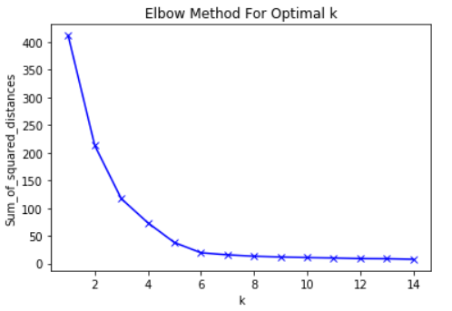
In cluster analysis, the elbow method is a heuristic used in determining the number of clusters in a data set. The method consists of plotting the explained variation as a function of the number of clusters, and picking the elbow of the curve as the number of clusters to use.

In this case the optimal clusters is 3, and 2 would be suboptimal.
Pros and Cons using K-Means
Pros :
- Simple to understand
- Fast to cluster
- Widely available
- Easy to implement
- Always yields a result
Cons (and Remedies) :
- Need to pick K (use the elbow method)
- Sensitive to initialization (use k-means++)
- Sensitive to outliers (just remove outliers)
- Produces spherical solutions
- Need to determine to use Standardization or not
K-Means Clustering in Python
We will be using sklearn.
Import the relevant libraries
1 | import pandas as pd |
Load the data
1 | # Load the clusters data |
Lets say we have this set of data.

^ Notice here Language is a Categorical Data. Thus we need to map the data.
Mapping Categoric Data
To map the data:
1 | data_mapped = data.copy() |
Plot the data
1 | # Use the simplest code possible to create a scatter plot using the longitude and latitude |
Select the features
DataFrame.iloc(row indices, column indices) slice the data frame, given rows and columns to e kept.
Example 1: We select Latitude and Longitude in this case.
1 | # iloc is a method used to 'slice' data |
Example2 : We select Language in this case.
1 | x2 = data_mapped.iloc[:,3:4] |
Example3: We select all both Latitude, Longitude and Language.
1 | x3 = data_mapped.iloc[:,1:4] |
Clustering
1 | # Create an object (which we would call kmeans) |
Show the Clustering results
1 | # Create a variable which will contain the predicted clusters for each observation |
Then plot the scatter plot
1 | # Plot the data using the longitude and the latitude |
Selecting the number of clusters
WCSS
1 | # Get the WCSS for the current solution |
Elbow Method
1 | # Create a variable containing the numbers from 1 to 6, so we can use it as X axis of the future plot |
K-Means Clustering in Python (Full Example)
In this example, I will be using the Iris flower dataset.
The Iris flower dataset is one of the most popular ones for machine learning. You can read a lot about it online and have probably already heard of it: https://en.wikipedia.org/wiki/Iris_flower_data_set
Import the relevant libraries
1 | import numpy as np |
Load the data
Load data from the csv file: ‘iris_dataset.csv’.
1 | # Load the data |

Plot the data
Try to cluster the iris flowers by the shape of their sepal.
Hint: Use the ‘sepal_length’ and ‘sepal_width’ variables.
1 | # Create a scatter plot based on two corresponding features (sepal_length and sepal_width; OR petal_length and petal_width) |
Clustering (unscaled data)
Separate the original data into 2 clusters.
1 | # create a variable which will contain the data for the clustering |
1 | # create a copy of data, so we can see the clusters next to the original data |
1 | # create a scatter plot based on two corresponding features (sepal_length and sepal_width; OR petal_length and petal_width) |
Standardize the variables (Scaling Data)
Import and use the scale function from sklearn to standardize the data.
1 | # import some preprocessing module |
Clustering (scaled data)
1 | # create a k-means object with 2 clusters |
1 | # create a copy of data, so we can see the clusters next to the original data |
1 | # create a scatter plot based on two corresponding features (sepal_length and sepal_width; OR petal_length and petal_width) |
Take Advantage of the Elbow Method
WCSS
1 | wcss = [] |
The Elbow Method
1 | number_clusters = range(1,cl_num) |
Based on the Elbow Curve, plot several graphs with the appropriate amounts of clusters you believe would best fit the data.
Understanding the Elbow Curve
Construct and compare the scatter plots to determine which number of clusters is appropriate for further use in our analysis. Based on the Elbow Curve, 2, 3 or 5 seem the most likely.
2 clusters
Start by seperating the standardized data into 2 clusters.
1 | kmeans_2 = KMeans(2) |
Construct a scatter plot of the original data using the standartized clusters.
1 | # Remember that we are plotting the non-standardized values of the sepal length and width. |
1 | plt.scatter(clusters_2['sepal_length'], clusters_2['sepal_width'], c= clusters_2 ['cluster_pred'], cmap = 'rainbow') |
3 Clusters
Redo the same for 3 and 5 clusters.
1 | kmeans_3 = KMeans(3) |
1 | clusters_3 = x.copy() |
1 | plt.scatter(clusters_3['sepal_length'], clusters_3['sepal_width'], c= clusters_3 ['cluster_pred'], cmap = 'rainbow') |
5 Clusters
1 | kmeans_5 = KMeans(5) |
1 | clusters_5 = x.copy() |
1 | plt.scatter(clusters_5['sepal_length'], clusters_5['sepal_width'], c= clusters_5 ['cluster_pred'], cmap = 'rainbow') |
Compare your solutions to the original iris dataset
The original (full) iris data is located in iris-with-answers.csv. Load the csv, plot the data and compare it with your solution.
Obviously there are only 3 species of Iris, because that’s the original (truthful) iris dataset.
The 2-cluster solution seemed good, but in real life the iris dataset has 3 SPECIES (a 3-cluster solution).
Therefore, clustering cannot be trusted at all times. Sometimes it seems like x clusters are a good solution, but in real life, there are more (or less).
1 | real_data = pd.read_csv('iris-with-answers.csv') |
1 | real_data['species'].unique() |
output: array(['setosa', 'versicolor', 'virginica'], dtype=object)
1 | # We use the map function to change any 'yes' values to 1 and 'no'values to 0. |
1 | real_data.head() |
Scatter plots (which we will use for comparison)
‘Real data’
Looking at the first graph it seems like the clustering solution is much more intertwined than what we imagined (and what we found before)
1 | plt.scatter(real_data['sepal_length'], real_data['sepal_width'], c= real_data ['species'], cmap = 'rainbow') |
Examining the other scatter plot (petal length vs petal width), we see that in fact the features which actually make the species different are petals and NOT sepals!
Note that ‘real data’ is the data observed in the real world (biological data)
1 | plt.scatter(real_data['petal_length'], real_data['petal_width'], c= real_data ['species'], cmap = 'rainbow') |
Our clustering solution data
It seems that our solution takes into account mainly the sepal features
1 | plt.scatter(clusters_3['sepal_length'], clusters_3['sepal_width'], c= clusters_3 ['cluster_pred'], cmap = 'rainbow') |
Instead of the petals…
1 | plt.scatter(clusters_3['petal_length'], clusters_3['petal_width'], c= clusters_3 ['cluster_pred'], cmap = 'rainbow') |
Further clarifications
In fact, if you read about it, the original dataset has 3 sub-species of the Iris flower. Therefore, the number of clusters is 3.
This shows us that:
- the Eblow method is imperfect (we might have opted for 2 or even 4)
- k-means is very useful in moments where we already know the number of clusters - in this case: 3
- biology cannot be always quantified (or better)… quantified with k-means! Other methods are much better at that
Finally, you can try to classify them (instead of cluster them, now that you have all the data)!
Hierarchical Clustering

There are two types of Hierarchical Clustering:
- Agglomerative (Bottom-up)
- each observation starts in its own cluster, and pairs of clusters are merged as one moves up the hierarchy, until all observations are in a single cluster.
- Divisive (Top-down)
- all observations are in the same cluster and then split into smaller clusters.
- To find the best split we must explore all possibilities at each step. (Elbow Methods)
We will focus on Agglomerative Clustering.
Agglomerative
Each observation starts in its own cluster, and pairs of clusters are merged as one moves up the hierarchy, until all observations are in a single cluster.
Dendrogram
The Agglomerative Graph is called Dendrogram.

In above example, 6 clusters -> 5 clusters left (Germany and France merged) -> 4 (UK and Germany and France merged) -> 3 (Canada and USA merged) -> 2 (UK and Germany and France and Canada and USA merged) -> 1 cluster in the end (Merge with Australia).
Note: All cluster solutions are nested inside the Dendrogram.
Pros of Dendrogram
- Hierarchical clustering shows all the possible linkages between clusters
- We understand the data much, much better
- No need to preset the number of clusters (like with k-means)
- Many methods the perform hierarchiclal clustering
Cons of Dendrogram
- Huge scaled obbservations will be extremely hard to be examined
HeatMap
Heatmap uses colors to represent a value.
Dendrogram and Heatmap in Python
Import the relevant libraries
1 | import numpy as np |
Load the data
pd.read_csv(*.csv,index_col) loads a given CSV file as a data frame; index_col is an argument which can specify a given column from the CSV as index of the data frame.
1 | # Load the standardized data |
1 | # Create a new data frame for the inputs, so we can clean it |
Plot the data
1 | # Using the Seaborn method 'clustermap' we can get a heatmap and dendrograms for both the observations and the features |
Reference
The Data Science Course 2020: Complete Data Science Bootcamp