Paper Review - T-Cell Receptor meets VAE

Prerequisite Knowledge

• VAE
  • Paper: Auto-Encoding Variational Bayes
  • Vines’ Log: Paper Review - Autoencoder (AE) and Variational Autoencoder (VAE)
• Wasserstein Distance
  • Vines’ Log: Overview on common Generative adversarial network methods

Domain Knowledge Terminologies

• Protein
  • a combination of 20 types of amino acids
• Peptide
  • a short sequence of amino acids
• Fold
  • refers to the specific three-dimensional arrangement (shape and surface characteristics) of a polypeptide chain. Crucial for the protein’s function.
• Pathogens
  • microorganisms that can cause disease
  • Types of Pathogens: Bacteria, Viruses, Fungi, Parasites…
• Antigens
  • Any substance that causes the body to make an immune response against that substance.
    • can be used as markers in laboratory tests to identify those tissues or cells.
  • Types of Antigens: toxins, chemicals, bacteria, viruses, or other substances that come from outside the body.
  • Body tissues and cells, including cancer cells, also have antigens on them that can cause an immune response.
• T-Cell
  • A type of immune cell that’s part of the body’s adaptive immune system, meaning it can learn to recognize and remember specific pathogens.
  • Kill cells that have been infected or mutated that may cause harm (e.g. cancer)
    • When to kill?
• T-Cell Receptor (TCR)
  • A molecule found on the surface of T-cells (A group of proteins found on T cells)
  • T-cell receptors bind to certain antigens (proteins) found on abnormal cells, cancer cells, cells from other organisms, and cells infected with a virus or another microorganism.
    • This interaction causes the T cells to attack these cells and helps the body fight infection, cancer, or other diseases.

Think of T-cells as security guards in a high-security facility (your body).

The T-cell receptor is like a specialized scanner each guard carries.

Just as a scanner helps identify unauthorized personnel or objects, the T-cell receptor helps the T-cell recognize and respond to invaders.

TCR-dWAE

Paper: Disentangled Wasserstein Autoencoder for T-Cell Receptor Engineering

Some parts of a protein are crucial for its function (like where it binds to other molecules), while other parts are important for maintaining its overall shape. But each part cannot work on its own without another part.

• Finding and changing the important functional parts is key for designing new proteins
  • Need to keep the overall structure while only functionally relevant part are changed for the efficiency
  • Challenging task because requires domain knowledge and limited to specific scenarios
• Proposed Wasserstein Autoencoder (WAE) + Auxiliary Classifier
  • to separate function and structure
  • Disentangled representation learning
    • similar to the content-style separation in computer vision and NLP problem
    • protein sequence separately embedded into a “functional” embedding and “structural” embedding
• Tested on T-cell Receptors because its a well-studied structure-function case
  • proposed method can alter the functions of TCR without changing the structural backbone
• First work to utilize disentangled representations for TCR Engineering

In practice, it is difficult to predict the real “structure” in the sense of protein 3D structure for CDR3beta region because it is a very flexible loop, and high-quality structure is scarce. Additionally, it cannot be predicted from the CDR3beta sequence alone, ignoring the rest of the TCR. Thus, we can only rely on the available sequential information of known CDR3beta’s to determine whether generated ones are valid, or whether they preserve the structural backbone, based on the intuition that the structure is defined by the sequence. Thus, if certain pivotal residues and motifs (which we try to make the “structural embedding” learn) are similar between two sequences (e.g. generated and known), they should have similar structures.

Problem Definition

Given A TCR sequence and a peptide that it could not bind to:

• Introduce a minimal number of mutations so that it can bind
• TCR needs to remain valid, with no major changes in the structural

TCRs that bind to the same peptide should have similar function patterns

• Focused on CDR3$\beta$ region of TCRs (the most active region for TCR binding)

The CDR3 (Complementarity-Determining Region 3) is a unique segment of the T-cell receptor. It plays a crucial role in recognizing and responding to antigens presented by antigen-presenting cells

(A) Top: The TCR recognizes antigenic peptides provided by the major histocompatibility complex (MHC) with high specificity; bottom: the 3D structure of the TCR-peptide-MHC binding interface (PDB: 5HHO); the CDRs are highlighted.

Method

Notation	Meaning
$\Theta_{f}$	functional encoder
$\Theta_{s}$	structural encoder
$\Gamma$	decoder
$\Psi$	auxiliary functional classifier
$\{\mathbf{x}, \mathbf{u}, y\}$	a data point with TCR $\mathbf{x}$, peptide $\mathbf{u}$ and binding label $y$
$\mathbf{z}_{f}$	functional embedding
$\mathbf{z}_{s}$	structural embedding
$\mathbf{z}$	concatenation of $\{\mathbf{z}_{f}, \mathbf{z}_{s}\}$
$\mathbf{x}'$	reconstructed/generated sequence from the decoder
$\mathbf{x}^{(i)}$	the probability distribution over amino acids at the $i$-th position in $\mathbf{x}$
$\text{concat}(\mathbf{x}_{1}, \ldots, \mathbf{x}_{n})$	concatenation of vectors $\{\mathbf{x}_{1}, \ldots, \mathbf{x}_{n}\}$

The disentangled autoencoder framework (WAE), where the input $x$, i.e., the CDR3β, is embedded into a functional embedding $z_f$ (orange bar) and structural embedding $z_s$ (green bar).

Architectures

Input sequences are padded to the same length (25). The peptide $u$ is presented as the average BLOSUM50 score for all its amino acids

• Embedding layer

  • tranform the one-hot encoded sequence x into continuous-valued vectors of 128 dim

• Trasnformer encoders as functional encoder $\Theta_{f}$ and structural encoder $\Theta_{s}$

  • 1 layer transformer with 8 attention heads and an intermediate size of 128
  • 2-layer MLP with a 128-dim hidden layer built on top of the transformer to transform the output to the dimensions of $z_f$ and $z_s$ respectively

• LSTM decoder as decoder $\Gamma$

  • 2-layer with 256 hidden dim

  • As our dataset is not very complex, we believe an LSTM is sufficient and is easier to implement. Also, in our application, there is only one embedding for the whole sequence, while a typical transformer decoder would accept token-wise embeddings. The latter may not be easily manipulated for sequence engineering.

• MLP as auxiliary functional classifier $\Psi$

  • 2-layer MLP with 32-dim hidden layer

WAE is trained deterministically, avoiding several practical challenges of VAE in general, especially on sequences.

• End-to-End training
• Trained with Adam Optim for 200 epochs, lr = 1e-4

Loss Functions

$$\mathcal{L} = \mathcal{L}_{\text{recon}} + \beta_1 \mathcal{L}_{c} + \beta_2\mathcal{L}_{wass}$$

• Binding Prediction Loss $\mathcal{L}_{c}$

  • Binary Cross Entropy (BCE)

• Reconstruction Loss $\mathcal{L}_{\text{recon}}$

  • Position-wise Binary Cross Entropy (BCE) across all positions of the sequence
  • $\beta_1 = 1.0$ in the paper

• Wasserstein autoencoder regularization $\mathcal{L}_{wass}$

  • by minimizing the MMD (maximum mean discrepancy) between the distribution of the embeddings and an isotropic multivariate Gaussian prior, so that $z_f$ and $z_s$ are independent.

    • embeddings $Z \sim Q_Z$ where $z = \text{concat}(z_f, z_s)$
    • isotropic multivariate Gaussian prior $Z_0 \sim P_Z$ where $P_Z = \mathcal{N}(0, I_d)$

  • $$MMD(P_Z, Q_Z) = \frac{1}{[n/2]}\sum^{[n/2]}_i h((z_{2i-1},\tilde{z}_{2i-1}),(z_{2i},\tilde{z}_{2i}))$$

    • where $h((z_{2i-1},\tilde{z}_{2i-1}),(z_{2i},\tilde{z}_{2i}) = k(z_i, z_j) + k(\tilde{z}_i, \tilde{z}_j) - k(z_i, \tilde{z}_j) - k(z_j, \tilde{z}_i)$ and $k$ is the RBF kernel function with $\sigma=1$.

  • $\beta_2 = 0.1$ in the paper

Inference

Method for sequence engineering with input $x$. structural embedding $z_s$ of the template sequence and a modified $z^′f$ functional embedding, are fed to the decoder to generate engineered TCRs $x'$

Disentanglement Guarantee

For some generative models, such as diffusion models, there is no “explicit” latent space. Methods like VAE and WAE “explicitly” model the distribution of the latent space, so we could directly enforce disentanglement on that latent space.

The measurement of disentanglement of the embeddings $Z_f$ and $Z_s$ given the variable $U$ (peptide).

$$D\left(\mathbf{Z}_f, \mathbf{Z}_s ; \mathbf{X} \mid \mathbf{U}\right)=V I\left(\mathbf{Z}_s ; \mathbf{X} \mid \mathbf{U}\right)+V I\left(\mathbf{Z}_f ; \mathbf{X} \mid \mathbf{U}\right)-V I\left(\mathbf{Z}_f ; \mathbf{Z}_s \mid \mathbf{U}\right)$$

where $VI$ is the variation of information, measuring of independence between two random variables.

the condition $U$ is omitted for the sake of simplicity.

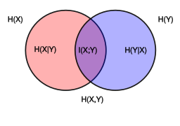
$$VI(X;Y\mid U) = H(X\mid U) + H(Y\mid U) - 2I(X;Y\mid U)\\ VI(X;Y) = H(X) + H(Y) - 2I(X;Y)$$

• $H$ is the Entropy
• $I$ is the Mutual Information

https://en.wikipedia.org/wiki/Mutual_information

This measurement reaches 0 when $Z_f$ and $Z_s$are totally independent, i.e. disentangled

Sub $VI(X;Y) = H(X) + H(Y) - 2I(X;Y)$ into $V I\left(\mathbf{Z}_s ; \mathbf{X} \right)+V I\left(\mathbf{Z}_f ; \mathbf{X} \right)-V I\left(\mathbf{Z}_f ; \mathbf{Z}_s \right)$, we get:

$$VI(\mathbf{Z}_s ; \mathbf{X} )+V I(\mathbf{Z}_f ; \mathbf{X} )-VI(\mathbf{Z}_f ; \mathbf{Z}_s) =H(Z_s) + H(X) - 2I(Z_s;X) + H(Z_f) + H(X) - 2I(Z_f;X) - H(Z_f) - H(Z_s) + 2I(Z_f;Z_s)$$

Cancelling out the terms:

$$V I\left(\mathbf{Z}_s ; \mathbf{X} \right)+V I\left(\mathbf{Z}_f ; \mathbf{X} \right)-V I\left(\mathbf{Z}_f ; \mathbf{Z}_s \right) = 2H(X) + 2[I(Z_f;Z_s) - I(Z_s;X) - I(Z_f;X)]$$

https://en.wikipedia.org/wiki/Data_processing_inequality
Data Processing Inequality

As $z_f \rightarrow x \rightarrow y$ forms a markov chain,

Using the mutual information, this can be written as :

$$I(x; z_f) \geq I(y; z_f)$$

Therefore we have the upper bound of the disentanglement objective (right hand side)

$$I(Z_f;Z_s) - I(Z_s;X) - I(Z_f;X) \leq I(Z_f;Z_s) - I(Z_s;X) - I(Z_f;Y)$$

Then we can minimize the whole upper bound term $\mathbf{I(Z_f;Z_s) - I(Z_s;X) - I(Z_f;Y)}$.

Maximizing $I(Z_s;X)$

Similar to Disentangled Recurrent Wasserstein Autoencoder

According to the Theorem, Given the encoder $Q_\theta(Z \mid X)$, decoder $P_\gamma(X \mid Z)$, prior $P(Z)$, and the data distribution $P_D$

$$\mathbb{D}_{K L}(Q(\mathbf{Z}) \| P(\mathbf{Z}))=\mathbb{E}_{p_D}\left[\mathbb{D}_{K L}\left(Q_\theta(\mathbf{Z} \mid \mathbf{X}) \| P(\mathbf{Z})\right)\right]-I(\mathbf{X} ; \mathbf{Z})$$

where $Q(Z)$ is the marginal distribution of the encoder when $X \sim P_D$ and $Z \sim Q_\theta (Z\mid X)$.

Proof:

Joint Generative Distribution:

$$p(\mathbf{x}, \mathbf{z}) = p_\gamma(\mathbf{x} \mid \mathbf{z})p(\mathbf{z})$$

Joint Inference Distribution:

$$q(\mathbf{x}, \mathbf{z}) = q_\theta(\mathbf{z}\mid \mathbf{x})p_D(\mathbf{x})$$

Now find $I(X; Z)$:

$$I(\mathbf{X} ; \mathbf{Z}) =\mathbb{E}_{q(\mathbf{x}, \mathbf{z})} \log \frac{q(\mathbf{x}, \mathbf{z})}{p_D(\mathbf{x}) q(\mathbf{z})}$$

Since $q(\mathbf{x}, \mathbf{z}) = q_\theta(\mathbf{z}\mid \mathbf{x})p_D(\mathbf{x})$, expend the term and cancel out $p_D(\mathbf{x})$

$$\mathbb{E}_{q(\mathbf{x}, \mathbf{z})} \log \frac{q(\mathbf{x}, \mathbf{z})}{p_D(\mathbf{x}) q(\mathbf{z})} = \mathbb{E}_{q(\mathbf{x}, \mathbf{z})} \log \frac{q_\theta(\mathbf{z}\mid \mathbf{x})p_D(\mathbf{x})}{p_D(\mathbf{x}) q(\mathbf{z})} = \mathbb{E}_{q(\mathbf{x}, \mathbf{z})} \log \frac{q_\theta(\mathbf{z}\mid \mathbf{x})}{q(\mathbf{z})}$$

Since $\mathbb{E}[XY] = \mathbb{E}[X]\mathbb{E}[Y]$ for independent variables $X, Y$, Using the formula we can decompose the joint expectation into the product of expectations $\mathbb{E}_{q(\mathbf{x}, \mathbf{z})} = \mathbb{E}_{p_D(x)}\mathbb{E}_{q_\theta(\mathbf{z}\mid \mathbf{x})}$.

For Conditional expectations, $\mathbb{E}[X|A] = \sum_x xP(X=x|A)$, so $\mathbb{E}_{q_\theta(\mathbf{z}\mid \mathbf{x})} = \sum_z q_\theta(\mathbf{z}\mid \mathbf{x})$

$$\mathbb{E}_{q(\mathbf{x}, \mathbf{z})} \log \frac{q_\theta(\mathbf{z}\mid \mathbf{x})}{q(\mathbf{z})} = \mathbb{E}_{p_D(x)}\mathbb{E}_{q_\theta(\mathbf{z}\mid \mathbf{x})} \log \frac{q_\theta(\mathbf{z}\mid \mathbf{x})}{q(\mathbf{z})} = \mathbb{E}_{p_D(x)} \sum_z q_\theta(\mathbf{z}\mid \mathbf{x}) \log \frac{q_\theta(\mathbf{z}\mid \mathbf{x})}{q(\mathbf{z})}$$

We need to rewrite this in a way that reflects both the joint distribution and marginal components. Rewrite the expectation to explicitly show $p_D(\mathbf{x})$ so once inside the summation and once inside the logarithm.

$$\mathbb{E}_{p_D(x)} \sum_z q_\theta(\mathbf{z}\mid \mathbf{x}) \log \frac{q_\theta(\mathbf{z}\mid \mathbf{x})}{q(\mathbf{z})} = \mathbb{E}_{p_D} \sum_{\mathbf{z}} q_\theta(\mathbf{z} \mid \mathbf{x}) \log \frac{q_\theta(\mathbf{z} \mid \mathbf{x}) p_D(\mathbf{x})}{p_D(\mathbf{x}) q(\mathbf{z})}$$

$$\mathbb{E}_{p_D} \sum_{\mathbf{z}} q_\theta(\mathbf{z} \mid \mathbf{x}) \log \frac{q_\theta(\mathbf{z} \mid \mathbf{x}) p_D(\mathbf{x})}{p_D(\mathbf{x}) q(\mathbf{z})}= \mathbb{E}_{p_D} \sum_{\mathbf{z}} p_D(\mathbf{x}) q_\theta(\mathbf{z} \mid \mathbf{x}) \log \frac{q_\theta(\mathbf{z} \mid \mathbf{x}) p_D(\mathbf{x})}{p_D(\mathbf{x}) q(\mathbf{z})}$$

Then cancel out the term $p_D(x)$

$$\mathbb{E}_{p_D} \sum_{\mathbf{z}} p_D(\mathbf{x}) q_\theta(\mathbf{z} \mid \mathbf{x}) \log \frac{q_\theta(\mathbf{z} \mid \mathbf{x}) p_D(\mathbf{x})}{p_D(\mathbf{x}) q(\mathbf{z})} = \mathbb{E}_{p_D} \sum_{\mathbf{z}} p_D(\mathbf{x}) q_\theta(\mathbf{z} \mid \mathbf{x}) \log \frac{q_\theta(\mathbf{z} \mid \mathbf{x})}{q(\mathbf{z})}$$

Since $p_D(x)$ is part of the expectation $\mathbb{E}_{p_D}$, we can factor it out of the summation

$$\mathbb{E}_{p_D} \sum_{\mathbf{z}} p_D(\mathbf{x}) q_\theta(\mathbf{z} \mid \mathbf{x}) \log \frac{q_\theta(\mathbf{z} \mid \mathbf{x}) }{q(\mathbf{z})} =\mathbb{E}_{p_D} \sum_{\mathbf{z}} q_\theta(\mathbf{z} \mid \mathbf{x}) \log \frac{q_\theta(\mathbf{z} \mid \mathbf{x})}{q(\mathbf{z})}$$

Using the logarithmic property $\log\frac{a}{b} = \log(\frac{a}{c}\times\frac{c}{b}) = \log(\frac{a}{c}/\frac{b}{c}) = \log\frac{a}{c} - \log\frac{b}{c}$:

$$\mathbb{E}_{p_D} \sum_{\mathbf{z}} q_\theta(\mathbf{z} \mid \mathbf{x}) \log \frac{q_\theta(\mathbf{z} \mid \mathbf{x})}{q(\mathbf{z})} =\mathbb{E}_{p_D} \sum_{\mathbf{z}} q_\theta(\mathbf{z} \mid \mathbf{x}) \log \frac{q_\theta(\mathbf{z} \mid \mathbf{x})}{p(\mathbf{z})}-\mathbb{E}_{p_D} \sum_{\mathbf{z}} q_\theta(\mathbf{z} \mid \mathbf{x}) \log \frac{q(\mathbf{z})}{p(\mathbf{z})} \\$$

$$=\mathbb{E}_{p_D} \sum_{\mathbf{z}} q_\theta(\mathbf{z} \mid \mathbf{x}) \log \frac{q_\theta(\mathbf{z} \mid \mathbf{x})}{p(\mathbf{z})}-\sum_{\mathbf{z}} q(\mathbf{z}) \log \frac{q(\mathbf{z})}{p(\mathbf{z})}$$

As the definition of KL divergence equation $\mathbb{D}_{\mathrm{KL}}(P\mid\mid Q) = \sum_iP(i)\log\frac{P(i)}{Q(i)}$

$$=\mathbb{E}_{p_D}\left[\mathbb{D}_{\mathrm{KL}}\left(Q_\theta(\mathbf{Z} \mid \mathbf{X}) \| P(\mathbf{Z})\right)\right]-\mathbb{D}_{\mathrm{KL}}(Q(\mathbf{Z}) \| P(\mathbf{Z}))$$

This final form is often used in variational inference, where it measures how well the conditional distribution $q_\theta(\mathbf{z} \mid \mathbf{x})$ fits the prior $p(z)$ on average, and compares this to the overall fit of the marginal $q(z)$ with respect to the prior.

Shortened version (From the paper):

$$\begin{aligned} I(\mathbf{X} ; \mathbf{Z}) & =\mathbb{E}_{q(\mathbf{x}, \mathbf{z})} \log \frac{q(\mathbf{x}, \mathbf{z})}{p_D(\mathbf{x}) q(\mathbf{z})} \\ & =\mathbb{E}_{p_D} \sum_{\mathbf{z}} p_D(\mathbf{x}) q_\theta(\mathbf{z} \mid \mathbf{x}) \log \frac{q_\theta(\mathbf{z} \mid \mathbf{x}) p_D(\mathbf{x})}{p_D(\mathbf{x}) q(\mathbf{z})} \\ & =\mathbb{E}_{p_D} \sum_{\mathbf{z}} q_\theta(\mathbf{z} \mid \mathbf{x}) \log \frac{q_\theta(\mathbf{z} \mid \mathbf{x})}{q(\mathbf{z})} \\ & =\mathbb{E}_{p_D} \sum_{\mathbf{z}} q_\theta(\mathbf{z} \mid \mathbf{x}) \log \frac{q_\theta(\mathbf{z} \mid \mathbf{x})}{p(\mathbf{z})}-\mathbb{E}_{p_D} \sum_{\mathbf{z}} q_\theta(\mathbf{z} \mid \mathbf{x}) \log \frac{q(\mathbf{z})}{p(\mathbf{z})} \\ & =\mathbb{E}_{p_D} \sum_{\mathbf{z}} q_\theta(\mathbf{z} \mid \mathbf{x}) \log \frac{q_\theta(\mathbf{z} \mid \mathbf{x})}{p(\mathbf{z})}-\sum_{\mathbf{z}} q(\mathbf{z}) \log \frac{q(\mathbf{z})}{p(\mathbf{z})} \\ & =\mathbb{E}_{p_D}\left[\mathbb{D}_{\mathrm{KL}}\left(Q_\theta(\mathbf{Z} \mid \mathbf{X}) \| P(\mathbf{Z})\right)\right]-\mathbb{D}_{\mathrm{KL}}(Q(\mathbf{Z}) \| P(\mathbf{Z})) \end{aligned}$$

Therefore by minimizing the KL divergence between the marginal $Q(Z)$ and the prior $P(Z)$, the mutual information $I(Z; X)$ is maximized.

Revisit KL Divergence:

• KL Divergence measures how different two probability distributions are from each other.
• Asymmetric (meaning the result changes if the distributions are switched.), KL(Q||P) does not equal to KL(P||Q).
• Log transformation is used to address biases in averaging large numbers.

This part corresponds to the training of Autoencoder. In practice, MMD (maximum mean discrepancy) between the distribution of the embeddings

Maximizing $I(Z_s;Y)$

$I(Z_s; Y)$ has a lower bound

$$I(Y; Z_f) = H(Y) - H(Y\mid Z_f) \\ I\left(Y ; \mathbf{Z}_f\right) \geq H(Y)+\mathbb{E}_{p\left(Y, \mathbf{Z}_f\right)} \log q_{\Psi}\left(Y \mid \mathbf{Z}_f\right)$$

Therefore maximizing the performance of classifier $\psi$ would maximize $I(Y; Z_f)$

Minimizing $I(Z_f; Z_s)$

By minimizing the Wasserstein loss between the distribution of the embeddings and an isotropic multivariate Gaussian prior, so that $z_f$ and $z_s$ are independent.

• Forces the embedding space $Z$ to approach an isotropic multivariate Gaussian prior $P_z = \mathcal{N}(0, I_d)$ where all the dimensions are independent

Minimizing the mutual information between the two parts of the embedding $Z_f$ and $Z_s$ is achieved by ensuring that the dimensions of $Z$ are independent.

Data Preparation

TCR-peptide interaction data from:

• VDJDB
• MCPAS

TCR-VALID

Paper: Designing meaningful continuous representations of T cell receptor sequences with deep generative models