Segmentation

What is Segmentation?

Partitioning images into different regions

Contours
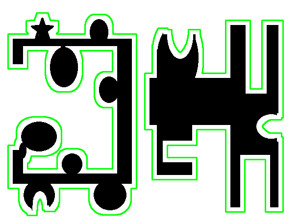
Contours are continuous lines or curves that bound or cover the full boundary of an object in an image.

Contours are very important in:

  • Object Detection
  • Shape Analysis

OpenCV stores Contours in a list of lists.

Code Implementation

cv2.findContours(image, Retrieval Mode, Approximation Method)

Reutrns contours, hierachy

NOTE In OpenCV 3.X, findContours returns a 3rd argument which is ret (or a boolean indicating if the function was successfully run).

If you’re using OpenCV 3.X replace line 19 with:

_, contours, hierarchy = cv2.findContours(image, cv2.RETR_EXTERNAL, cv2.CHAIN_APPROX_NONE)

The variable ‘contours’ are stored as a numpy array of (x,y) points that form the contour

While, ‘hierarchy’ describes the child-parent relationships between contours (i.e. contours within contours)

1
2
3
4
5
6
7
8
9
10
11
12
13
14
15
16
17
18
19
20
21
22
23
24
25
26
27
28
29
30
31
import cv2
import numpy as np

# Let's load a simple image with 3 black squares
image = cv2.imread('images/shapes.jpg')
cv2.imshow('Input Image', image)
cv2.waitKey(0)

# Grayscale
gray = cv2.cvtColor(image,cv2.COLOR_BGR2GRAY)

# Find Canny edges
edged = cv2.Canny(gray, 30, 200)
cv2.imshow('Canny Edges', edged)
cv2.waitKey(0)

# Finding Contours
# Use a copy of your image e.g. edged.copy(), since findContours alters the image
contours, hierarchy = cv2.findContours(edged, cv2.RETR_EXTERNAL, cv2.CHAIN_APPROX_NONE)[-2:]
cv2.imshow('Canny Edges After Contouring', edged)
cv2.waitKey(0)

print("Number of Contours found = " + str(len(contours)))

# Draw all contours
# Use '-1' as the 3rd parameter to draw all
cv2.drawContours(image, contours, -1, (0,255,0), 3)

cv2.imshow('Contours', image)
cv2.waitKey(0)
cv2.destroyAllWindows()

Hierarchy Types:

  • cv2.RETR_LIST - Retrieves all contours
  • cv2.RETR_EXTERNAL - Retrieves external or outer contours only
  • cv2.RETR_COMP - Retrieves all in a 2-level hierarchy
  • cv2.RETR_TREE - Retrieves all in full hierarchy

Sorting Contours

Suprisingly useful technique when applying object recognition algorithms or machine learning classification algorithms.

Sorting by Area can assist in Object Recognition (using contour area)

  • Eliminate small contours that may be noise
  • Extract the largest contour

Sorting by spatial position (using contour centroid)

  • Sort characters left to right
  • Process images in specific order

Before Sorting

1
2
3
4
5
6
7
8
9
10
11
12
13
14
15
16
17
18
19
20
21
22
23
24
25
26
27
28
29
30
31
32
33
34
35
36
37
import cv2
import numpy as np

# Load our image
image = cv2.imread('images/bunchofshapes.jpg')
cv2.imshow('0 - Original Image', image)
cv2.waitKey(0)

# Create a black image with same dimensions as our loaded image
blank_image = np.zeros((image.shape[0], image.shape[1], 3))

# Create a copy of our original image
orginal_image = image

# Grayscale our image
gray = cv2.cvtColor(image,cv2.COLOR_BGR2GRAY)

# Find Canny edges
edged = cv2.Canny(gray, 50, 200)
cv2.imshow('1 - Canny Edges', edged)
cv2.waitKey(0)

# Find contours and print how many were found
contours, hierarchy = cv2.findContours(edged.copy(), cv2.RETR_EXTERNAL, cv2.CHAIN_APPROX_NONE)[:2]
print ("Number of contours found = ", len(contours))

#Draw all contours
cv2.drawContours(blank_image, [contours], -1, (0,255,0), 3)
cv2.imshow('2 - All Contours over blank image', blank_image)
cv2.waitKey(0)

# Draw all contours over blank image
cv2.drawContours(image, contours, -1, (0,255,0), 3)
cv2.imshow('3 - All Contours', image)
cv2.waitKey(0)

cv2.destroyAllWindows()

Sorting by Area

1
2
3
4
5
6
7
8
9
10
11
12
13
14
15
16
17
18
19
20
21
22
23
24
25
26
27
28
29
30
31
32
33
34
35
36
import cv2
import numpy as np

# Function we'll use to display contour area

def get_contour_areas(contours):
# returns the areas of all contours as list
all_areas = []
for cnt in contours:
area = cv2.contourArea(cnt)
all_areas.append(area)
return all_areas

# Load our image
image = cv2.imread('images/bunchofshapes.jpg')
orginal_image = image

# Let's print the areas of the contours before sorting
print("Contor Areas before sorting")
print(get_contour_areas(contours))

# Sort contours large to small
sorted_contours = sorted(contours, key=cv2.contourArea, reverse=True)
#sorted_contours = sorted(contours, key=cv2.contourArea, reverse=True)[:3]

print("Contor Areas after sorting")
print(get_contour_areas(sorted_contours))

# Iterate over our contours and draw one at a time
for c in sorted_contours:
cv2.drawContours(orginal_image, [c], -1, (255,0,0), 3)
cv2.waitKey(0)
cv2.imshow('Contours by area', orginal_image)

cv2.waitKey(0)
cv2.destroyAllWindows()

Sorting by spatial position

1
2
3
4
5
6
7
8
9
10
11
12
13
14
15
16
17
18
19
20
21
22
23
24
25
26
27
28
29
30
31
32
33
34
35
36
37
38
39
40
41
42
43
44
45
46
47
48
49
50
51
52
53
54
55
56
57
58
59
60
61
62
import cv2
import numpy as np

# Functions we'll use for sorting by position

def x_cord_contour(contours):
#Returns the X cordinate for the contour centroid
if cv2.contourArea(contours) > 10:
M = cv2.moments(contours)
return (int(M['m10']/M['m00']))
else:
pass


def label_contour_center(image, c):
# Places a red circle on the centers of contours
M = cv2.moments(c)
cx = int(M['m10'] / M['m00'])
cy = int(M['m01'] / M['m00'])

# Draw the countour number on the image
cv2.circle(image,(cx,cy), 10, (0,0,255), -1)
return image


# Load our image
image = cv2.imread('images/bunchofshapes.jpg')
orginal_image = image.copy()


# Computer Center of Mass or centroids and draw them on our image
for (i, c) in enumerate(contours):
orig = label_contour_center(image, c)

cv2.imshow("4 - Contour Centers ", image)
cv2.waitKey(0)

# Sort by left to right using our x_cord_contour function
contours_left_to_right = sorted(contours, key = x_cord_contour, reverse = False)


# Labeling Contours left to right
for (i,c) in enumerate(contours_left_to_right):
cv2.drawContours(orginal_image, [c], -1, (0,0,255), 3)
M = cv2.moments(c)
cx = int(M['m10'] / M['m00'])
cy = int(M['m01'] / M['m00'])
cv2.putText(orginal_image, str(i+1), (cx, cy), cv2.FONT_HERSHEY_SIMPLEX, 1, (0, 255, 0), 2)
cv2.imshow('6 - Left to Right Contour', orginal_image)
cv2.waitKey(0)
(x, y, w, h) = cv2.boundingRect(c)

# Let's now crop each contour and save these images
cropped_contour = orginal_image[y:y + h, x:x + w]
image_name = "output_shape_number_" + str(i+1) + ".jpg"
print(image_name)
cv2.imwrite(image_name, cropped_contour)

cv2.destroyAllWindows()


Approximating Contours and Convex Hull

Approximating Contours

cv2.approxPolyDP(contour, Approximation Accuracy, Closed)

  • contour – is the individual contour we wish to approximate
  • Approximation Accuracy – Important parameter is determining the accuracy of the approximation. Small values give precise- approximations, large values give more generic approximation. A good rule of thumb is less than 5% of the contour perimeter
  • Closed – a Boolean value that states whether the approximate contour should be open or closed
1
2
3
4
5
6
7
8
9
10
11
12
13
14
15
16
17
18
19
20
21
22
23
24
25
26
27
28
29
30
31
32
33
34
import numpy as np
import cv2

# Load image and keep a copy
image = cv2.imread('images/house.jpg')
orig_image = image.copy() # backup the image
cv2.imshow('Original Image', orig_image)
cv2.waitKey(0)

# Grayscale and binarize
gray = cv2.cvtColor(image, cv2.COLOR_BGR2GRAY)
ret, thresh = cv2.threshold(gray, 127, 255, cv2.THRESH_BINARY_INV)

# Find contours
contours, hierarchy = cv2.findContours(thresh.copy(), cv2.RETR_LIST, cv2.CHAIN_APPROX_NONE)

# Iterate through each contour and compute the bounding rectangle
for c in contours:
x,y,w,h = cv2.boundingRect(c)
cv2.rectangle(orig_image,(x,y),(x+w,y+h),(0,0,255),2)
cv2.imshow('Bounding Rectangle', orig_image)

cv2.waitKey(0)

# Iterate through each contour and compute the approx contour
for c in contours:
# Calculate accuracy as a percent of the contour perimeter
accuracy = 0.03 * cv2.arcLength(c, True)
approx = cv2.approxPolyDP(c, accuracy, True)
cv2.drawContours(image, [approx], 0, (0, 255, 0), 2)
cv2.imshow('Approx Poly DP', image)

cv2.waitKey(0)
cv2.destroyAllWindows()

Convex Hull

1
2
3
4
5
6
7
8
9
10
11
12
13
14
15
16
17
18
19
20
21
22
23
24
25
26
27
import numpy as np
import cv2

image = cv2.imread('images/hand.jpg')
gray = cv2.cvtColor(image, cv2.COLOR_BGR2GRAY)

cv2.imshow('Original Image', image)
cv2.waitKey(0)

# Threshold the image
ret, thresh = cv2.threshold(gray, 176, 255, 0)

# Find contours
contours, hierarchy = cv2.findContours(thresh.copy(), cv2.RETR_LIST, cv2.CHAIN_APPROX_NONE)

# Sort Contors by area and then remove the largest frame contour
n = len(contours) - 1
contours = sorted(contours, key=cv2.contourArea, reverse=False)[:n]

# Iterate through contours and draw the convex hull
for c in contours:
hull = cv2.convexHull(c)
cv2.drawContours(image, [hull], 0, (0, 255, 0), 2)
cv2.imshow('Convex Hull', image)

cv2.waitKey(0)
cv2.destroyAllWindows()

Shape Matching

Find most similar shape.

cv2.matchShapes(contour template, contour, method, method parameter)

Output – match value (lower values means a closer match)

  • Contour Template – This is our reference contour that we’re trying to find in the new image
  • Contour – The individual contour we are checking against
  • Method – Type of contour matching (1, 2, 3)
  • Method Parameter – leave alone as 0.0 (not fully utilized in python OpenCV)
1
2
3
4
5
6
7
8
9
10
11
12
13
14
15
16
17
18
19
20
21
22
23
24
25
26
27
28
29
30
31
32
33
34
35
36
37
38
39
40
41
42
43
44
import cv2
import numpy as np

# Load the shape template or reference image
template = cv2.imread('images/4star.jpg',0)
cv2.imshow('Template', template)
cv2.waitKey()

# Load the target image with the shapes we're trying to match
target = cv2.imread('images/shapestomatch.jpg')
target_gray = cv2.cvtColor(target,cv2.COLOR_BGR2GRAY)

# Threshold both images first before using cv2.findContours
ret, thresh1 = cv2.threshold(template, 127, 255, 0)
ret, thresh2 = cv2.threshold(target_gray, 127, 255, 0)

# Find contours in template
contours, hierarchy = cv2.findContours(thresh1, cv2.RETR_CCOMP, cv2.CHAIN_APPROX_SIMPLE)

# We need to sort the contours by area so that we can remove the largest
# contour which is the image outline
sorted_contours = sorted(contours, key=cv2.contourArea, reverse=True)

# We extract the second largest contour which will be our template contour
template_contour = contours[1]

# Extract contours from second target image
contours, hierarchy = cv2.findContours(thresh2, cv2.RETR_CCOMP, cv2.CHAIN_APPROX_SIMPLE)

for c in contours:
# Iterate through each contour in the target image and
# use cv2.matchShapes to compare contour shapes
match = cv2.matchShapes(template_contour, c, 3, 0.0)
print(match)
# If the match value is less than 0.15 we
if match < 0.15:
closest_contour = c
else:
closest_contour = []

cv2.drawContours(target, [closest_contour], -1, (0,255,0), 3)
cv2.imshow('Output', target)
cv2.waitKey()
cv2.destroyAllWindows()

Identify Shapes by Contours

1
2
3
4
5
6
7
8
9
10
11
12
13
14
15
16
17
18
19
20
21
22
23
24
25
26
27
28
29
30
31
32
33
34
35
36
37
38
39
40
41
42
43
44
45
46
47
48
49
50
51
52
53
54
55
56
57
58
59
60
61
62
63
64
65
66
67
68
69
70
71
72
73
74
75
76
77
import numpy as np
import cv2

# Load and then gray scale image

image = cv2.imread('images/someshapes.jpg')
gray = cv2.cvtColor(image, cv2.COLOR_BGR2GRAY)

cv2.imshow('Identifying Shapes',image)
cv2.waitKey(0)

ret, thresh = cv2.threshold(gray, 127, 255, 1)

# Extract Contours
contours, hierarchy = cv2.findContours(thresh.copy(), cv2.RETR_LIST, cv2.CHAIN_APPROX_NONE)

for cnt in contours:

# Get approximate polygons
approx = cv2.approxPolyDP(cnt, 0.01*cv2.arcLength(cnt,True),True)

if len(approx) == 3:
shape_name = "Triangle"
cv2.drawContours(image,[cnt],0,(0,255,0),-1)

# Find contour center to place text at the center
M = cv2.moments(cnt)
cx = int(M['m10'] / M['m00'])
cy = int(M['m01'] / M['m00'])
cv2.putText(image, shape_name, (cx-50, cy), cv2.FONT_HERSHEY_SIMPLEX, 1, (0, 0, 0), 1)

elif len(approx) == 4:
x,y,w,h = cv2.boundingRect(cnt)
M = cv2.moments(cnt)
cx = int(M['m10'] / M['m00'])
cy = int(M['m01'] / M['m00'])

# Check to see if 4-side polygon is square or rectangle
# cv2.boundingRect returns the top left and then width and
if abs(w-h) <= 3:
shape_name = "Square"

# Find contour center to place text at the center
cv2.drawContours(image, [cnt], 0, (0, 125 ,255), -1)
cv2.putText(image, shape_name, (cx-50, cy), cv2.FONT_HERSHEY_SIMPLEX, 1, (0, 0, 0), 1)
else:
shape_name = "Rectangle"

# Find contour center to place text at the center
cv2.drawContours(image, [cnt], 0, (0, 0, 255), -1)
M = cv2.moments(cnt)
cx = int(M['m10'] / M['m00'])
cy = int(M['m01'] / M['m00'])
cv2.putText(image, shape_name, (cx-50, cy), cv2.FONT_HERSHEY_SIMPLEX, 1, (0, 0, 0), 1)

elif len(approx) == 10:
shape_name = "Star"
cv2.drawContours(image, [cnt], 0, (255, 255, 0), -1)
M = cv2.moments(cnt)
cx = int(M['m10'] / M['m00'])
cy = int(M['m01'] / M['m00'])
cv2.putText(image, shape_name, (cx-50, cy), cv2.FONT_HERSHEY_SIMPLEX, 1, (0, 0, 0), 1)


elif len(approx) >= 15:
shape_name = "Circle"
cv2.drawContours(image, [cnt], 0, (0, 255, 255), -1)
M = cv2.moments(cnt)
cx = int(M['m10'] / M['m00'])
cy = int(M['m01'] / M['m00'])
cv2.putText(image, shape_name, (cx-50, cy), cv2.FONT_HERSHEY_SIMPLEX, 1, (0, 0, 0), 1)

cv2.imshow('Identifying Shapes',image)
cv2.waitKey(0)

cv2.destroyAllWindows()

Line Detection

ρ=xcosθ+ysinθ\rho = xcos\theta + ysin\theta

where ρ\rho is the perpendicular distance from origin, θ\theta is the angle formed by the normal of this line to the origin (measured in radians)

There are 2 algorithms available in OpenCV.

Hough Lines

cv2.HoughLines(binarized/thresholded image, 𝜌 accuracy, 𝜃 accuracy, threshold)

  • Threshold here is the minimum vote for it to be considered a line
1
2
3
4
5
6
7
8
9
10
11
12
13
14
15
16
17
18
19
20
21
22
23
24
25
26
27
28
29
30
import cv2
import numpy as np

image = cv2.imread('images/soduku.jpg')

# Grayscale and Canny Edges extracted
gray = cv2.cvtColor(image, cv2.COLOR_BGR2GRAY)
edges = cv2.Canny(gray, 100, 170, apertureSize = 3)

# Run HoughLines using a rho accuracy of 1 pixel
# theta accuracy of np.pi / 180 which is 1 degree
# Our line threshold is set to 240 (number of points on line)
lines = cv2.HoughLines(edges, 1, np.pi / 180, 240)

# We iterate through each line and convert it to the format
# required by cv.lines (i.e. requiring end points)
for rho, theta in lines[0]:
a = np.cos(theta)
b = np.sin(theta)
x0 = a * rho
y0 = b * rho
x1 = int(x0 + 1000 * (-b))
y1 = int(y0 + 1000 * (a))
x2 = int(x0 - 1000 * (-b))
y2 = int(y0 - 1000 * (a))
cv2.line(image, (x1, y1), (x2, y2), (255, 0, 0), 2)

cv2.imshow('Hough Lines', image)
cv2.waitKey(0)
cv2.destroyAllWindows()

Probabilistic Hough Lines

The idea is that it takes only a random subset of points sufficient enough for line detection.

Also returns the start and end points of the line unlike the previous function

cv2.HoughLinesP(binarized image, 𝜌 accuracy, 𝜃 accuracy, threshold, minimum line length, max line gap)

1
2
3
4
5
6
7
8
9
10
11
12
13
14
15
16
17
18
19
20
21
import cv2
import numpy as np

# Grayscale and Canny Edges extracted
image = cv2.imread('images/soduku.jpg')
gray = cv2.cvtColor(image, cv2.COLOR_BGR2GRAY)
edges = cv2.Canny(gray, 100, 170, apertureSize = 3)

# Again we use the same rho and theta accuracies
# However, we specific a minimum vote (pts along line) of 100
# and Min line length of 5 pixels and max gap between lines of 10 pixels
lines = cv2.HoughLinesP(edges, 1, np.pi / 180, 200, 5, 10)

print(lines.shape)

for x1, y1, x2, y2 in lines[0]:
cv2.line(image, (x1, y1), (x2, y2),(0, 255, 0), 3)

cv2.imshow('Probabilistic Hough Lines', image)
cv2.waitKey(0)
cv2.destroyAllWindows()

Circle Detection

cv2.HoughCircles(image, method, dp, MinDist, param1, param2, minRadius, MaxRadius)

  • Method - currently only cv2.HOUGH_GRADIENT available
  • dp - Inverse ratio of accumulator resolution
  • MinDist - the minimum distance between the center of detected circles
  • param1 - Gradient value used in the edge detection
  • param2 - Accumulator threshold for the HOUGH_GRADIENT method (lower allows more circles to be detected (false positives))
  • minRadius - limits the smallest circle to this size (via radius)
  • MaxRadius - similarly sets the limit for the largest circles
1
2
3
4
5
6
7
8
9
10
11
12
13
14
15
16
17
18
19
20
21
22
23
24
import cv2
import numpy as np
import cv2.cv as cv

image = cv2.imread('images/bottlecaps.jpg')
gray = cv2.cvtColor(image, cv2.COLOR_BGR2GRAY)

blur = cv2.medianBlur(gray, 5)

circles = cv2.HoughCircles(blur, cv.CV_HOUGH_GRADIENT, 1.5, 10)
#circles = cv2.HoughCircles(gray, cv.CV_HOUGH_GRADIENT, 1, 10)

circles = np.uint16(np.around(circles))

for i in circles[0,:]:
# draw the outer circle
cv2.circle(image,(i[0], i[1]), i[2], (255, 0, 0), 2)

# draw the center of the circle
cv2.circle(image, (i[0], i[1]), 2, (0, 255, 0), 5)

cv2.imshow('detected circles', image)
cv2.waitKey(0)
cv2.destroyAllWindows()

Blob Detection

What is a Blob?

Blobs can be described as groups of connected pixels that all share a common property.

How to use OpenCV’s simpleBlob Detector?

  1. Create Detector
  2. Input image into Detector
  3. Obtain Key points
  4. Draw Key points

Code Implementation

cv2.drawKeypoints(input image, keypoints, blank_output_array, color, flags)

flags:

  • cv2.DRAW_MATCHES_FLAGS_DEFAULT
  • cv2.DRAW_MATCHES_FLAGS_DRAW_RICH_KEYPOINTS
  • cv2.DRAW_MATCHES_FLAGS_DRAW_OVER_OUTIMG
  • cv2.DRAW_MATCHES_FLAGS_NOT_DRAW_SINGLE_POINTS
1
2
3
4
5
6
7
8
9
10
11
12
13
14
15
16
17
18
19
20
21
22
23
24
# Standard imports
import cv2
import numpy as np;

# Read image
image = cv2.imread("images/Sunflowers.jpg")

# Set up the detector with default parameters.
detector = cv2.SimpleBlobDetector()

# Detect blobs.
keypoints = detector.detect(image)

# Draw detected blobs as red circles.
# cv2.DRAW_MATCHES_FLAGS_DRAW_RICH_KEYPOINTS ensures the size of
# the circle corresponds to the size of blob
blank = np.zeros((1,1))
blobs = cv2.drawKeypoints(image, keypoints, blank, (0,255,255),
cv2.DRAW_MATCHES_FLAGS_DEFAULT)

# Show keypoints
cv2.imshow("Blobs", blobs)
cv2.waitKey(0)
cv2.destroyAllWindows()

Blob Filtering

Blob filtering - Sape & Size

cv2.SimpleBlobDetector_Params()

Usage :

1
params = cv2.SimpleBlobDetector_Params()

Area

  • params.filterByArea = True/False
  • params.minArea = pixels
  • params.maxArea = pixels

Circularity

  • params.filterByCircularity= True/False
  • params.minCircularity = 1 being perfect circle, 0 the opposite

Convexity – Area of blob / Area of Convex Hull

  • params.filterByConvexity = True/False
  • params.minConvexity = 0 to 1

Inertia – Measure of ellipticalness (low being more elliptical, high being more circular)

  • params.filterByInertia = True/False
  • params.minInertiaRatio = 0.01

Object Detection

Object Detection is very important in computer vision.

What for?

  • Labeling Scenes
  • Robot Navigation
  • Self Driving Cars
  • Body Recognition (Microsoft Kinect)
  • Disease & Cancer Detection
  • Facial Recognition
  • Handwriting Recognition
  • Identifying objects in satellite images etc.

Object Detection vs Recognition

What is the difference?

Object Detection

Only looks at one particular object and does not try to recognize exactly what it seeing.

Recognition

Recognition is basically the second level of object detection.

It allows the computer to actually recognize multiple objects within an image.

Template Matching

This method isn’t very resilient.

  • Rotation renders this method ineffective
  • Size (Scaling) affects this as well
  • Photometric changes (brigntness, contrast, hue etc.)
  • Distortions from view point changes (Affine)

Interest Points (Image Features)

Image Features are interesting areas of an image that are somewhat unique to that specific image.

Also called key point features or interest points

Why Important?

Features are important as they can be used to analyze, describe and match images.

Features are used in:

  • Image Alignment
  • 3D Reconstruction
  • Robot Navigation
  • Object Recognition
  • Motion Tracking etc.

What Interesting?

Interesting areas carry a lot of distinct and unique information at that point

  • High change of intensity
  • Corners or edges

Be careful that noise can appear informative.

Characteristics

Repeatable

  • Can be found in multiple pictures of the same scene

Distinctive

  • Each feature is somewhat unique and different and other features of the same scene

Compactness/Efficiency

  • Significantly less features than pixels in the image

Locality

  • Feature occupies a small area of the image and is robust to clutter and occlusion

Corners as Features

Corners are identified when shifting a window in any direction over that point gives a large change in intensity.

Best summaries images in terms of image matching

  • Flat - No Intensity change in any direction
  • Edge - Intensity change in one direction
  • Corner - Intensity change in all directions

Code Implementation

Harros Corner Detection

Harris Corner Detection is an algorithm developed in 1998 for corner detection and works fairly well

cv2.cornerHarris(input image, block size, ksize, k)

  • Input image - should be grayscale and float32 type.
  • blockSize - the size of neighborhood considered for corner detection
  • ksize - aperture parameter of Sobel derivative used.
  • k - harris detector free parameter in the equation
  • Output – array of corner locations (x,y)
1
2
3
4
5
6
7
8
9
10
11
12
13
14
15
16
17
18
19
20
21
22
import cv2
import numpy as np

# Load image then grayscale
image = cv2.imread('images/chess.jpg')
gray = cv2.cvtColor(image, cv2.COLOR_BGR2GRAY)

# The cornerHarris function requires the array datatype to be float32
gray = np.float32(gray)

harris_corners = cv2.cornerHarris(gray, 3, 3, 0.05)

#We use dilation of the corner points to enlarge them\
kernel = np.ones((7,7),np.uint8)
harris_corners = cv2.dilate(harris_corners, kernel, iterations = 2)

# Threshold for an optimal value, it may vary depending on the image.
image[harris_corners > 0.025 * harris_corners.max() ] = [255, 127, 127]

cv2.imshow('Harris Corners', image)
cv2.waitKey(0)
cv2.destroyAllWindows()

Good Features to Track

Good Features to Track is a better algorithm for corner dectection.

cv2.goodFeaturesToTrack(input image, maxCorners, qualityLevel, minDistance)

  • Input Image - 8-bit or floating-point 32-bit, single-channel image.
  • maxCorners – Maximum number of corners to return. If there are more corners than are found, the strongest of them is returned.
  • qualityLevel – Parameter characterizing the minimal accepted quality of image corners. The parameter value is multiplied by the best corner quality measure (smallest eigenvalue). The corners with the quality measure less than the product are rejected. For example, if the best corner has the quality measure = 1500, and the qualityLevel=0.01 , then all the corners with the quality - - measure less than 15 are rejected.
  • minDistance – Minimum possible Euclidean distance between the returned corners.
1
2
3
4
5
6
7
8
9
10
11
12
13
14
15
16
17
18
import cv2
import numpy as np

img = cv2.imread('images/chess.jpg')
gray = cv2.cvtColor(img,cv2.COLOR_BGR2GRAY)

# We specific the top 50 corners
corners = cv2.goodFeaturesToTrack(gray, 100, 0.01, 150)

for corner in corners:
x, y = corner[0]
x = int(x)
y = int(y)
cv2.rectangle(img,(x-10,y-10),(x+10,y+10),(0,255,0), 2)

cv2.imshow("Corners Found", img)
cv2.waitKey()
cv2.destroyAllWindows()

Problems with corners as features

Tolerant of:

  • Rotations
  • Translations (e.g. Shifts in image)
  • Slight photometric changes (e.g. brightness or affine intensity)

Intolerant of:

  • Lage Intensity changes or photometric changes
  • Scaling issues

SIFT

SIFT (Scale Invariant Feature Transform)

Note: SIFT is patented and no longer freely available with OpenCV 3.0+.

It is free to use for academic and research purposes :) Try older versions of OpenCV for SIFT.

Basically what SIFT do

  1. Detect interesting key points in an image using the difference of gaussian method
  2. Create vector descriptor for these interesting areas.
  3. Scale invariance is achieved by
    1. Scanning interest points at several different scales
    2. The scale which meet a specific stability criteria is selected and endcoded by the vector descriptor
    3. Regardless of the initial size, the most stable scale is found which allows us to be scale invariant
  4. Rotation invariance is achieved by obtaining the Orientation Assignment of the key point using image gradient magnitudes
  5. Once we know the 2D direction, we can normalize this direction.

SURF

SURF (Speeded Up Robbust Features)

SURF was developed to improve the speed of a scale invariant feature detector.

Basically what SURF do

  1. Use Hessian matrix approximation to detect interesting points
  2. Use the sum of Haar wavelet responses for orientation assignment

Alternatives to SIFT and SURF

FAST

FAST (Features from Accelerated Segment Test)

  • Key point detection only (no descriptor)
  • Used in real time applications

BRIEF

BRIEF (Binary Robust Independent Elementary Features)

  • Fast
  • Computers descriptors quickly (instead of using SIFT or SURF)

ORB

ORB (Oriented FAST and Rotated BRIEF)

  • Combines both FAST and BRIEF
  • Free to use (Developed out of OpenCV)

Histogram of Oriented Gradients

Histogram of Oriented Gradients (HOGs) are a feature descriptor that has been widely and successfully used for object detection.

  • represents objects as a single feature vector as opposed to a set of feature vectors where each represents a segment of image
  • computed by sliding window detector over an image, where a HOG descriptor is a computed for each position.
  • often used with SVM (support vector machine) classifiers. Each HOS descriptor that is computed is fed to a SVM classifier to determine if the object was found or not.

Basically what HOGs do

E.g. There is a picture 64×12864 \times 128 pixels.

  1. Using an 8x8 pixel detection window or cell, we compute the gradient vector or edge orientations at each pixel.
  2. This generates 64 (8x8) gradient vectors which are then represented as a histogram.
  3. Each cell is then split into angular bins, where each bin corresponds to a gradient direction (e.g. x,y). 9 bins are used in this case.
  4. The effectively reduces 64 vectors to just 9 values.
  5. As it stores gradients magnitudes, it;'s relatively immune to deformations
  6. We then Normalize the gradients to ensure invariance to illumination changes (i.e. Brightness and Contrast).
  7. Instead of individual window cell normalization, a method called Block Normalization is used
  8. Block Normalization takes into account neighboring blocks so we normalize taking into consideration lager segments of the image.