Fundamentals of Digital Image Processing

Interest in digital image processing methods stems from 2 principal application areas:

improvement of pictorial information for human interpretation
processing of scene data for autonomous machine perception
- extacting from an image information in a form suitable for computer processing

More specific application examples:

Acquire an image

Correct aperture and color balance

Reconstruct image from projections

Prepare for display or printing

Adjust image size

Color mapping, gamma-correction, halftoning

Facilitate picture storage and transmission

Efficiently store an image in a digital camera

Send an image from space

Enhance and restore images

Touch up personal photos

Color enhancement for security screening

Extract information from images

Read 2-d bar codes

Character recognition

Many more … image processing is ubiquitous

What is an Image?

An image refers to a 2D light intensity function $f(x,y)$ .

Where

$(x,y)$ denote spatial coordinates
$f(x,y)$ is a value proportional to the brightness or gray levels of the image at that point.

A digital image is an image $f(x,y)$ that has been discretized both in spatial coordinates and brightness. Each element of such a digital array is called a pixel or a pel.

To be suitable for computer processing, an image $f(x,y)$ must be digitalized both spatially and in amplitude.

Digitization of the spatial coordinates (x,y) is called image sampling.

Amplitude digitization is called gray-level quantization.

$\text{Aspect ratio} = \frac{\text{no. of columns}}{\text{no. of rows}}$

$\text{Spatial resolution} = \frac{\text{no. of columns} \times \text{no. of rows}}{inch}$

$\text{Amplitude resolution (a.k.a. bit depth)} = \frac{\text{bits}}{\text{pixel}}$

The storage and processing requirements increase rapidly with the spatial resolution and the number of gray levels.

Example: A 256 gray-level image of size 256x256 occupies 64K bytes of memory

$256 \times 256 = 64 \times 2^{10} = 64K \space \text{bytes}$

Example: A color image is in raw RGB format. Its bit depth is 12 bits per color component and its spatial resolution is $1024\times480$ . How many bytes are required to store this image if no compression is performed?

$w \times h \times 3 \text{channel} \times 12\text{bits} = 36wh \space \text{bits}$

$\frac{1024\times480\times12\times3}{8} = 2160 \times 2^{10} = 2160K \space \text{bytes} = 2211840 \space \text{bytes}$

Fundamental steps in Image Processing

Image acquisition -> Image preprocessing -> Image segmentation -> Image representation -> Image description -> Image recognition -> Image interpretation

Knowledge about a problem domain is coded into an image processing system in the form of a knowledge database.

Image Processing is Application-oriented.

Image acquisition

to acquire a digital image

Image preprocessing

to improve the image in ways that increase the chances for success of the other processes.

Image segmentation

to partitions an input image into its constituent parts or objects.
E.g. Segment the picture into regions. Each region contains only one object for easier processing.

Image representation

to convert the input data to a form suitable for computer processing.
E.g. Normalization of size and orientation. Contour approximation to remove unnecessary details

Image description

to extract features that result in some quantitative information of interest or features that are basic for differentiating one class of objects from another.
E.g. Feature vector extraction

Image recognition

to assign a label to an object based on the information provided by its descriptors.

Image interpretation

to assign meaning to an ensemble of recognized objects.

Elements of digital Image processing systems

The basic operations performed in a digital image processing systems includes:

1: acquisition
2: storage
3: processing
4: communnication
5: display

Color processing

Visible Lights

Color is the perceptual result of light in the visible region of the spectrum, having in the region of 400nm to 700nm, incident upon the retina. Visible Light is a form of electromagnetic energy consisting of a spectrum of frequencies having wavelengths range from about 400nm for violet light to about 700nm for red light. Most light we see is a combination of many wavelengths.

3 basic qualities are used to describe the quality of a chromatic light source:

Radiance: the total amount of energy that flows from the light source (measured in watts)

Luminance: the amount of energy an observer perceives from the light source (measured in lumens)

Note we can have high radiance, but low luminance

Brightness: a subjective (practically unmeasurable) notion that embodies the intensity of light

RGB Model

RGB is an additive color model that generates colors by combining blue, green and red and different intensities/brightness.

Each colour appears in its primary spectral components of R, G and B

A 3-D Cartesian co-ordinate system
All axis are normalized to the range of 0 to 1
The Grayscale (Points of equal RGB values) extends from origin to farthest point
Different colors are points on or inside the cube

Images comprise 3 independent image plances (each for R,G,B respectively.)

The number of bits representing each pixel in RGB space is called pixel depth

Each R,G,B image is an 8-bit image
Each RGB color pixel has a depth of 24 bits - full-color image.
The total number of colors = 256 x 256 x 256 = 16,777,216

Example:

The Bit Depth of a grey-level image is 4. Mark all its possible pixel colors in the RGB space.

$2^4 = 16$

The 16 Points equally divide the straight line connecting (0,0,0) Black and (1,1,1) White.

The RGB coordinates are in a form of ( $\frac{k}{15}$ , $\frac{k}{15}$ , $\frac{k}{15}$ ) where $k \in (0,1,2,3,4,5,6,7,8,9,10,11,12,13,14,15)$

CMY Model

CMY model, which uses Cyan, Magenta and Yellow primaries, is mostly used in printing devices where the color pigments on the paper absorb certain colors.

Cyan is the compliment of Red
Magenta is the compliment of Green
Yello is the compliment of Blue

$\left[\begin{array}{c} C \\ M \\ Y \end{array}\right]=\left[\begin{array}{c} 1-R \\ 1-G \\ 1-B \end{array}\right]$

Sometimes, an alternative CMYK model is used in color printing to produce a darker black than simply mixing CMY.

$\left[\begin{array}{c} C^{\prime} \\ M^{\prime} \\ Y^{\prime} \end{array}\right]=\left[\begin{array}{c} C-K \\ M-K \\ Y-K \end{array}\right]$

Where K = min{C,M,Y}

Primaries

Any color can be matched by proper proportions of three component colors called primaries.

The most common primaries are red, blue and green.

Subject Emits Light -> Additive Mixing

Subject Does not Emit Light -> Subtractive Mixing

When Two complementary colors of each other mixed together in equal intensities, White color is produced.

$\text{Red} + \text{Cyan} = \text{Red} + (\text{Green} + \text{Blue}) = \text{White}$

$\text{Blue} + \text{Yellow} = \text{Blue} + (\text{Green} + \text{Red}) = \text{White}$

$\text{Green} + \text{Magenta} = \text{Green} + (\text{Red} + \text{Blue}) = \text{White}$

$\text{Cyan} = \text{White} - \text{Red}$

$\text{Yellow} = \text{White} - \text{Blue}$

$\text{Magenta} = \text{White} - \text{Green}$

Examples:

What color would a white paper appear when exposed to red light?

Material reflects R, G and B & there is only R → Red

What color would a red paper appear when exposed to yellow light?

Material only reflects R & there are R and G → Red

What color would a cyan paper appear when exposed to yellow light?

Material reflects G and B & there are R and G → Green

What color would a magenta paper appear when exposed to white light?

Material reflects R and B & there are R, G and B → R & B = Magenta

What color would a blue paper appear when exposed to red light?

Material only reflects B & there is only R → Black

^ Rules :

Look at Addivtive primaries.

When a Material Reflect $\{X\}$ Colors, and Expose to $\{Y\}$ Colors Light,

Material would appear $\{X \cap Y\}$ Color. (If $\{X\}$ and $\{Y\}$ has no intersection, Black Color appear.)

Example:

(a) RGB

(Brighter = Higher value of that Color)

Fig.Q4b is Red channel

Fig.Q4c is Green channel

Fig.Q4d is Blue channel

(b) CMYK

(Brighter = Higher value of that Color)

Fig Q4f is Magenta channel

Fig Q4g is Yellow channel

Fig Q4h is Cyan channel

Fig Q4e is Black channel

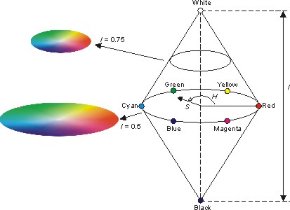
HSI Color Space

The HSI color space is very important and attractive color model for image processing applications because it represents colors similarly how the human eye senses colors. The HSI color model represents every color with three components: hue ( H ), saturation ( S ), intensity ( I ).

Hue, saturation and brightness are basic elements in defining a color.

Hue indicates the color spectrum (color)
Saturation indicates the spectral purity of the color in the light

HSI stands for Hue, Saturation and Intensity.

It decouples the intensity component from the color-carrying information (hue and saturation) in a color.

What is the difference between HSI and HSV color space?

RGB to HSI transformation:

Learn more about Conversion from RGB to HSI here!

$H=\left\{\begin{array}{ccc} \theta & \text {if } \quad B \leq G \\ 2 \pi-\theta & \text { if } \quad B>G \end{array}\right.$

$\text { where } \quad \theta=\cos ^{-1}\left\{\frac{\frac{1}{2}[(R-G)+(R-B)]}{\left[(R-G)^{2}+(R-B)(G-B)\right]^{1 / 2}}\right\}$

$S=1-\frac{3}{R+G+B}[\min (R, G, B)]$

$I=\frac{1}{3}(R+G+B)$

It is good practice to add a small number in the denominator of the θ expression to avoid dividing by 0 when R = G = B, in which case θ will be 90°.

$cos^{-1}(0) = 90°$

Example:

Given 3 Colors whose RGB representations are given as follows:

Color A: (0.5, 0.5, 0.5)

Color B: (0.4, 0.6, 0.5)

Color C: (0.3, 0.7, 0.5)

(a) Which Color does not carry chrominance (Color) Information?

Saturation indicates the spectral purity of the color in the light (Chrominance)

Color A: (0.5, 0.5, 0.5) -> H = 90°, S = 0, I = 0.5 -> S=0, No Chrominance Information

(b) Which Color has a Stronger Luminance (Intensity of Light)?

Color B: (0.4, 0.6, 0.5) -> I = 0.5

Color C: (0.3, 0.7, 0.5) -> I = 0.5

All color has a same Luminance.

Color C is biased to middle of Green and Cyan ( or just Green among R, G and B)

CIE Chromacity Diagram

In 1931, the International Commission on Illumination (CIE) adopted a set of nonphysical primaries, X, Y and Z. It is a device-invariant representation of color. It serves as a standard reference for defining other color spaces.

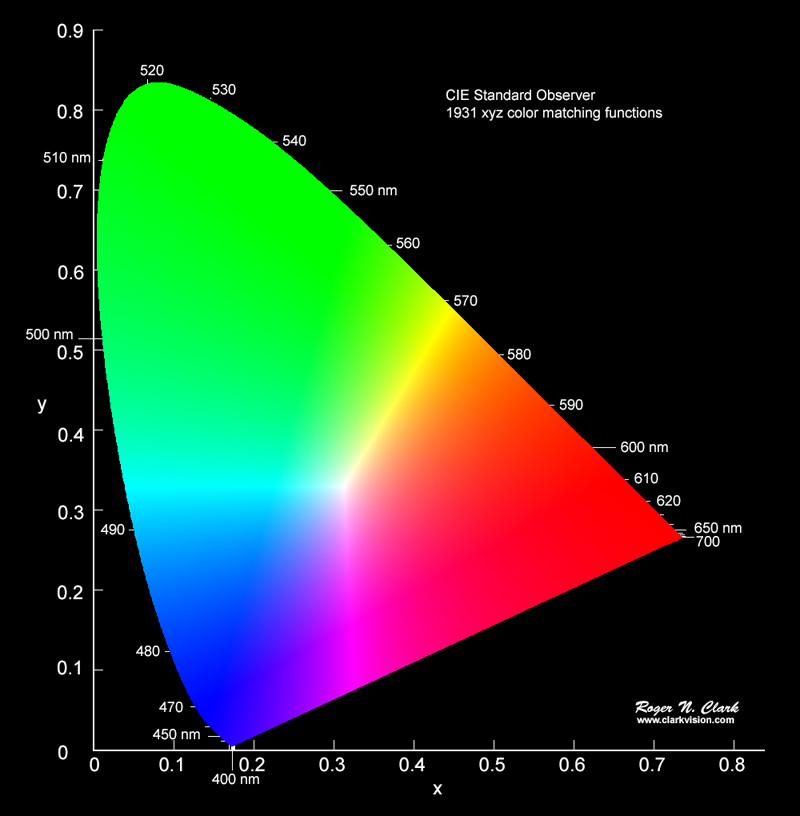
The amounts of R, G, B needed to form any particular colour are called the tristimulus values X, Y, and Z.

The CIE primary Y is carefully arranged such that it determines the luminance (brightness) of the colour.

$\left[\begin{array}{l} X \\ Y \\ Z \end{array}\right]=[M]\left[\begin{array}{l} R \\ G \\ B \end{array}\right]$

A colour is specified by its trichromatic coefficients:

$x = \frac{X}{X+Y+Z}$

$y = \frac{Y}{X+Y+Z}$

$z = \frac{Z}{X+Y+Z}$

$x+y+z = 1$

A colour can therefore be specified by its chromaticity and luminance in an (x, y, Y) triplet. Here, x and y are the chromaticity coordinates.

The edges represent the “pure” colors (i.e. fully saturated).

Any straight line joining two points in the diagram defines all of the different colors that can be obtained by combining these two colors additively.

Applications of common Color Models

Some common models used in popular applications:

For Display:
- RGB color model
For Printing:
- CMY or CMYK color model
For Storage (Compression) of Image:
- YUV and YIQ color model
For Storage (Compression) of Video:
- YUV, YIQ and YCbCr color model

We have covered Display and Printing models, now we will cover the storage models.

Chroma Subsampling

Chroma subsampling is a type of compression that reduces the color information in a signal in favor of luminance data. This reduces bandwidth without significantly affecting picture quality. More Info Here.

YIQ Color Model

Both YUV and YIQ Color Model are commonly used for storage.

For color TV boardcasting, which is downward compatible with B/W TV where only Y is used.

Luminance information is carried by Y
Chrominance (Color) information is carried by I and Q

Chrominance is relatively not as important as luminance and hence U and V components are generally downsampled before storing the image (Chroma subsampling).

YUV (YCbCr) Color Model

Both YUV and YIQ Color Model are commonly used for storage.

Initally for PAL analog video, but it’s now used in CCIR 601 standard for digital video.

Luminance information is carried by Y
Chrominance (Color) information is carried by U and V

Chrominance is relatively not as important as luminance and hence U and V components are generally downsampled before storing the image (Chroma subsampling).

Types of Chroma Subsampling

4:2:2 - Horizontally subsampled color signals by a factor of 2.
4:1:1 - Horizontally subsample by a factor of 4
4:2:0 - Subsampled in both the horizonal and vertical axes by a factor of 2 between pixels

4:1:1 and 4:2:0 are mostly used in JPEG and MPEG.

Example of Chroma Subsampling 4:1:1 by averaging

First Convert RGB into YCbCr

Image Enhancement

The principal objective of image enhancement is to process a given image so that the result is more suitable than the original image for a specific application. It accentuates or sharpens image features such as edges, boundaries, or contrast to make a graphic display more helpful for display and analysis.

The enhancement doesn’t increase the oringinal information content of the data, but it increases the dynamic range of the chosen features so that they can be detected easily.

There are many ways to enhance image in the spatial domain.

Simple intensity transformation
Histogram processing
Spatial filtering

There are also way to enhace image in frequency domain.

Lowpass / Highpass Filtering

The greatest difficulty in image enhancement is quantifying the criterion for enhancement and, therefore, a large number of image enhancement techniques are empirical and require interactive procedures to obtain satisfactory results. As mentioned above, Image enhancement methods can be based on either spatial or frequency domain techniques.

Enhancement in the spatial domain

Spatial domain techniques are

performed to the image plane itself
and based on direct manipulation of pixels in an image

The operation can be formulated as

$g(x,y) = T[f(x,y)]$

where $g$ is the output, $f$ is the input image and $T$ is an operation on $f$ defined over some neighborhood of (x,y).

The neighborhood about a point (x,y) can be defined using a square or rectangle sub-image area (also called window) centered at (x,y). The center of neighborhood sliding from top left to right every row and apply $T$ operation each location.

Simple Intensity transformation

$T$ is a scalar to scalar mapping.

Image negatives

Negatives of digital images are useful in numerous applications, for example:

Displaying medical images
Transformation between positive and negative films

$g(x,y) = L - f(x,y)$

Where $L$ is the max. intensity.

Contrast stretching

Use to increase the dynamic range of the gray levels in the image being processed
can be used to improve the contrast of an image

Low-contrast images can result from

poor illumination,

lack of dynamic range in the image sensor, or

even wrong setting of a lens aperture during image acquisition.

The idea behind contrast stretching is to increase the dynamic range of the gray levels in the image being processed.

Compression of dynamic range

Sometimes the dynamic range of a processed image far exceeds the capability of the display device, in which case only the brightest/darkest parts of the images are visible on the display screen

An effective way to compress the dynamic range of pixel values

$s = c \space ln(1 + |r|)$

where c is a scaling constant, and the logarithm function performs the desired compression.

Example:

Gray-level slicing

Highlighting a specific range of gray levels in an image often is desired.

Applications include: enhancing features such as masses of water in satellite imagery, and enhancing flaws in x-ray images.

The 2 Examples of Gray-level slicing:

A transformation function that highlights a range of intensities while diminishing all others to a constant.

A transformation function that highlights a range of intensities but preserves all others.

Power-law transformation

A variety of devices used for image capture, printing and display respond accordingly to a power law, which should be corrected and the correction process is called gamma correction.

$s = c r^\gamma$

where $c$ and $\gamma$ > 0, $0 \leq r \leq 1$

If $s$ is normalized to be in $[0,1]$ $\rightarrow$ $c=1$

A gamma value $\gamma <1$ is sometimes called an encoding gamma, and the process of encoding with this compressive power-law nonlinearity is called gamma compression.
conversely a gamma value $\gamma >1$ is called a decoding gamma, and the application of the expansive power-law nonlinearity is called gamma expansion.

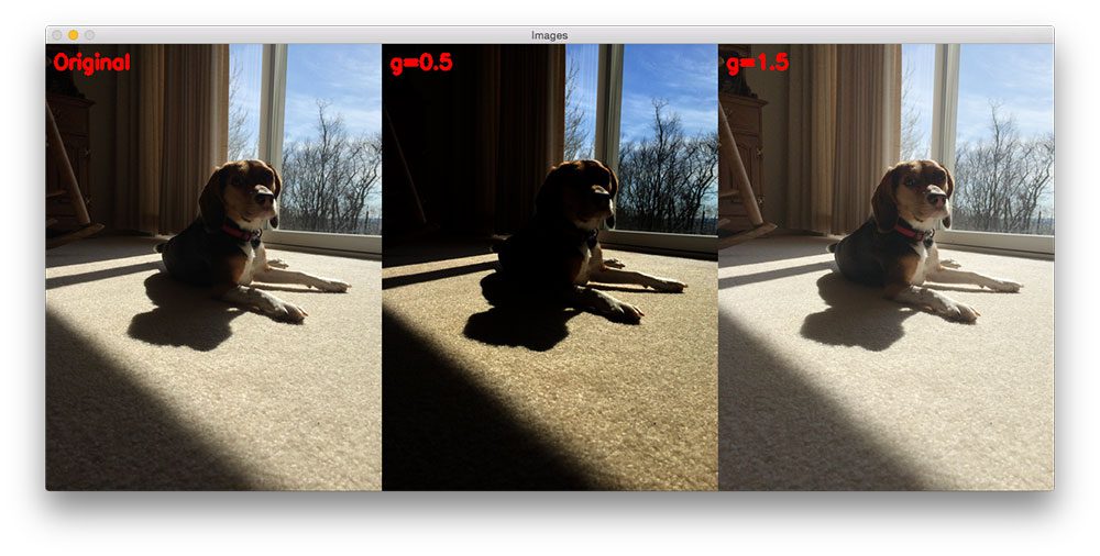
In real life, when we take a photo, the sunlight maybe too bright / too dark to cause the image unclear. Therefore we need gamma correction.

Gamma correction can be performed by pre-processing the input image with the transformation before inputting it into the systems.

Histogram processing

$T$ is a scalar-to-scalar mapping defined based on the pixel distribution of the whole image.

The histogram of a digital image with gray levels in the range $[0,L-1]$ is a discrete function

$p(r_k)=\frac{n_k}{n}$

where

$r_k$ is the kth gray level
$n_k$ is the number of pixels in the image with that gray level
$n$ is the total number of pixels in the image
$k$ =0,1…L-1.

$p(r_k)$ gives an estimate of the proability of occurrence of gray level $r_k$ .

Usage of Histogram

The shape of the histogram of an image gives us useful information about the possibility for contrast enhancement.
A histogram of a narrow shape indicates little dynamic range and thus corresponds to an image having low contrast.

Histogram equalization

Also known as histogram linearization.

can be used to improve the contrast of an image
To map an input image to an output image such that its histogram is uniform after the mapping.
Let $r$ represent the gray levels in the image to be enhanced and $s$ is the enhanced output with a transformation.

$s_k = T(r_k) = \sum^k_{j=0}\frac{n_j}{n}$

where $k = 0,1...L-1$

Note:

$T(r)$ is single-valued and monotonically increasing in the interval [0,1], which preserves the order from black to white in the gray scale.

$0\leq T(r) \leq 1$ for $0\leq r \leq 1$ , which guarantees the mapping is consistent with the allowed range of pixel values.

Example: Violation

Try sub $r_1 = 0$ and $r_2 = 1$ into the intensity mapping function T:

$z_1 = 1 - 0$

$z_2 = 1 - 1$

Therefore $r_1 = 0, r_2 = 0, z_1 = 1, z_2 = 0$ .

This violate the rule of histogram equalization because the mapping must be consistant. (if $r_1$ < $r_2$ , $z_1$ should also be < $z_2$ )

Example: Equalinzing an image of 6 gray levels:

Local enhancement

It is often necessary to enhance details over small areas.

The number of pixels in these areas may have negligible influence on the computation of a global transformation, so the use of global histogram specification does not necessarily guarantee the desired local enhancement.

Prcedures:

Define a square or rectangular neighborhood and move the center of this window from pixel to pixel.
Determine the histogram equalization or histogram specification transformation function with the histogram of the windowed image at each location.
Map the gray level centers in the window with the transformation function.
Move to an adjacent pixel location and the procedure is repeated.

Image before and after local enhancement:

Spatial Filtering

$T$ is a vector-to-scalar mapping. Can be linear (e.g. LPF) or non-linear (e.g. median filtering).

Spatial filtering can be a linear or non-linear process.

The use of spatial masks for image processing is called spatial filtering.
The masks used are called spatial filters and the values of a mask are referred to as filter coefficients.

The basic implementation of linear spatial filtering is 2D convolution.

$R(x, y)=\sum_{i=-d}^{d} \sum_{j=-d}^{d} w(i, j) f(x-i, y-j)$

where:

$(2d+1)\times(2d+1)$ is the mask size,
$w(i,j)$ are weights of the mask,
$f(x,y)$ is the input pixel at coordinates (x,y),
$R(x,y)$ is the output value at (x,y).

Note:

For outbounded window:

we ignore the number in deep learning’s 2DCONV approach, but now we are not doing deep learning 2DCONV approach.

Here we copy the values of nearest grid.

Smoothing Filters (blurring and noise reduction)

Smoothing filters are used for blurring and for noise reduction.

Blurring is used in preprocessing steps, such as removal of small details (noise!) from an image prior to object extraction, and bridging of small gaps in lines or curves.
Noise reduction can be accomplishing by blurring with a linear filter and also by nonlinear filtering.

Low pass filtering

It blurs edges and other sharp details in the image.

all coefficients must be positive
Neighborhood averaging is a special case of LPF where all coefficients are equal
blurs edges and other sharp details in the image.

Example: Averaging filter

$\frac{1}{9}\left[\begin{array}{lll} 1 & 1 & 1 \\ 1 & 1 & 1 \\ 1 & 1 & 1 \end{array}\right]$

General Formula:

$\frac{1}{\sum_{i=1}^9 n_i}\left[\begin{array}{lll} n_1 & n_2 & n_3 \\ n_4 & n_5 & n_6 \\ n_7 & n_8 & n_9 \end{array}\right]$

Median filtering

If the objective is to achieve noise reduction instead of blurring, this method should be used.

This method is particularly effective when the noise pattern consists of strong, spike-like components and the characteristic to be preserved is edge sharpness.

Median filtering is good at removing spike noise, but not so at removing white noise.

It is a nonlinear operation.

For each input pixel f(x,y), we sort the values of the pixel and its neighbors to determine their median and assign its value to output pixel g(x,y).

Next, the values are rounded.

Sharpening Filters (highlight fine detail)

Sharpening Filters are used to highlight fine detail in an image or to enhance detail that has been blurred, either in error or as a natural effect of a particular method of image acquisition.

to highlight fine detail in an image
to enhance detail that has been blurred

Uses of image sharpening vary and include applications ranging from electronic printing and medical imaging to industrial inspection and autonomous target detection in smart weapons.

Basic highpass spatial filter

The shape of the impulse response needed to implement a highpass spatial filter indicates that the filter should have positive coefficients near its center, and negative coefficients in the outer periphery.

Example:

$\frac{1}{9}\left[\begin{array}{ccc} -1 & -1 & -1 \\ -1 & 8 & -1 \\ -1 & -1 & -1 \end{array}\right]$

The filtering output pixels might be of a gray level exceeding [0,L-1].

The results of highpass filtering involve some form of scaling and/or clipping to make sure that the gray levels of the final results are within [0,L-1].

Derivative filter

Differentiation can be expected to have the opposite effect of averaging, which tends to blur detail in an image, and thus sharpen an image and be able to detect edges.

The most common method of differentiation in image processing applications is the gradient.

For a function f(x,y), the gradient of f at coordinates (x’,y’) is defined as the vector

$\nabla f\left(x^{\prime}, y^{\prime}\right)=\left[\begin{array}{l} \frac{\partial f}{\partial x} \\ \frac{\partial f}{\partial y} \end{array}\right]_{\left(x^{\prime}, y^{\prime}\right)}$

Its magnitude can be approximated in a number of ways, which result in a number of operators such as Roberts, Prewitt and Sobel operators for computing its value.

Enhancement in the frequency domain

These methods enhance an image f(x,y) by convoluting the image with a linear, position invariant operator.

The 2D convolution is performed in frequency domain with DFT (Discrete Fourier Transform).

Frequency Domain:

$G(w_1,w_2) = F(w_1,w_2)H(w_1,w_2)$

Lowpass Filtering

Edges and sharp transitions in the gray levels contribute to the high frequency content of its Fourier transform, so a lowpass filter smoothes an image.

can effectively remove random noise, but not salt noise

Formula of ideal LPF

$H(u, v)=\left\{\begin{array}{cc} 1 & \text { if } D(u, v) \leq D_{o} \\ 0 & \text { else } \end{array}\right.$

Highpass Filtering

A highpass filter attenuates the low frequency components without disturbing the high frequency information in the Fourier transform domain can sharpen edges.

Formula of ideal HPF

$H(u, v)=\left\{\begin{array}{cc} 0 & \text { if } D(u, v) \leq D_{o} \\ 1 & \text { else } \end{array}\right.$