Images

What are Images?

2-Dimensional representation of the visble light spectrum
Each pixel point corresponds to a different color which means that reflects different wavelengths of light

How are images formed?

When light reflects off an object at different points and bounces off onto a film, sensor or retina
Essentially use a barrier to block off most points of light while leaving a small gap (aperture)
Aperture allows some points of light to be reflected onto the film

a simple pinhole camera model

A simple pinhole camera model (Above image) and the aperture is always fixed. So that means that a constant amount of light is always entering this hall which can be sometimes overpowering for the film. Meaning that everything is going to look white.

Therefore It need to be fixed. See below explaination!

Controlling Image Formation with a Lens

Both our eyes and camera use an adaptive lens to control many aspects of image formation:

Aperture Size
- Controls the amount of light allowed through ( f-stops in cameras)
- Depth of Field (Bokeh)
Lens width
- Adjust focus distance (near of far)

Using Lens

How Human see images?

The human visual system (eye & visual cortex) is incredibly good at image processing.

They’re remarkably good at focusing quickly seeing in varying light conditions and picking up sharp details and then in terms of it to printing what we see humans are exceptional at this as we can quickly understand the context of different images and quickly identify objects faces you name it we can actually do this far better than any computer vision technique right now.

Our brains do this by using six layers of visual processing.

How do Computer store images?

Computer use RGB color space by default. What is RGB?
Each pixel corrdinate (x,y) of a 2D plane contains 3 values ranging for intensities of 0 to 255 (8-bit).
- Red
- Green
- Blue

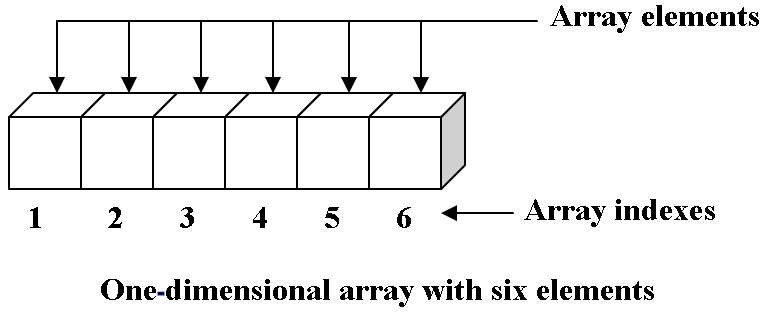
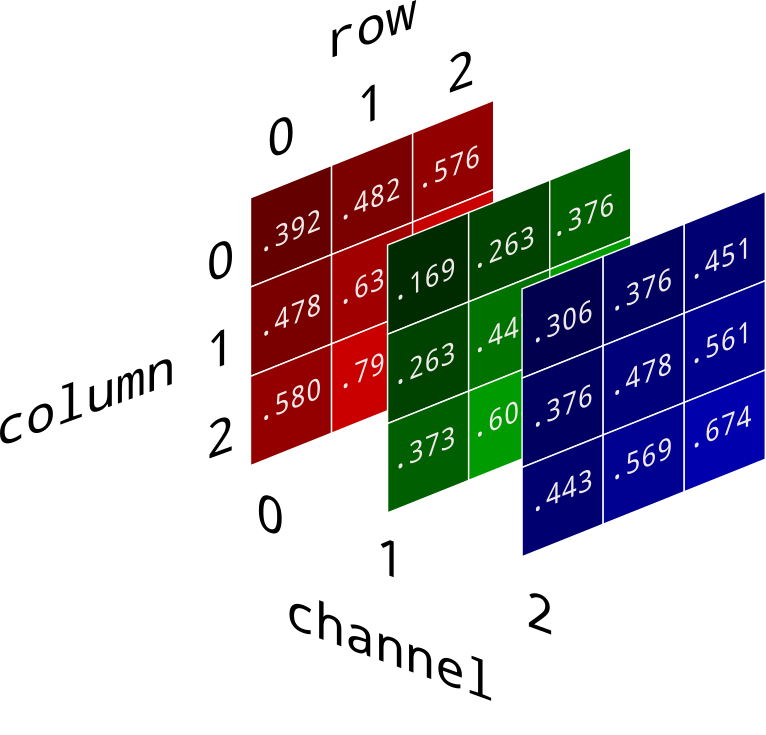
Images are stored in multi-dimensional arrays

1-dimensional array

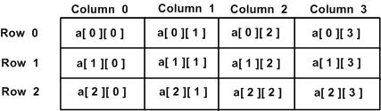
2-dimensional array

Think of it like an x y coordinate system.

3-dimensional array <- Where images are stored

Think of this as many two dimensional arrays stacked together.

Black and White or Greyscale

Black and White images are stored in 2-Dimensional arrays.
Two Types of B&W images :
- Grayscale - Ranges of shades of grey (255 - 0)
- Binary - Pixels are either black or white (255 or 0)

OpenCV

What is OpenCV?

OpenCV (Open Source Computer Vision) is a library of programming functions mainly aimed at real-time computer vision. Originally developed by Intel, it was later supported by Willow Garage then Itseez. The library is cross-platform and free for use under the open-source BSD license.

You can use either C++ or Python with it.

OpenCV in Python

Why Python?

Python allows us to do to easily grasp complex concepts.
Python is one of the easiest easiest languages for beginners
It is extremely powerful for data science and machine learning applications
It stores images in numpy arrays which allows us to do some very powerful operations quite easily

Checking my OpenCV version

# Import OpenCV
import cv2

# Print my OpenCV version
cv2.__version__

Loading and Displaying a Image

# Import OpenCV
import cv2

# Load an image using 'imread' specifying the path to image
image = cv2.imread('./images/Z.jpg')
# ^Opening the images inside the folder called `images` at the same location

# To display our image using `imshow`-> image show
cv2.imshow('Megaman Zero', image)


# `waitKey` allows us to input information when a image window is open
# By leaving it blank it just waits for anykey to be pressed before continuing.
# By placing numbers (except 0), we can specify a delay
# for how long you keep the window open (time is in milliseconds)
cv2.waitKey(0)

# Very Important! This closes all open windows
cv2.destroyAllWindows()
# ^Failure to place this will result in program crash

ok, lets try the code

import cv2
image = cv2.imread('./images/Z.jpg')
cv2.imshow('Megaman Zero', image)
cv2.waitKey(0)
cv2.destroyAllWindows()

Getting Info of the Image

To take a closer look at how images are stored, we need to use numpy.

# Import numpy
import numpy as np

# Get the dimensions of the image array
print image.shape
# ^It should return 3 values. The last value '3' means we are using RGB values

# Let's print each dimension of the image
print('Height of Image:', int(image.shape[0]), 'pixels')
print('Width of Image:', int(image.shape[1]), 'pixels')

Save Images We Edit in OpenCV

1
2
3

# Use 'imwrite' specificing the file name and the image to be saved (generated)
cv2.imwrite('output.jpg', image)
#^ If the image is generated successfully, it will return true.

Which IDE should I use?

Normal IDEs

import cv2
cv2.__version__
import numpy as np
image = cv2.imread('./images/Z.jpg')
cv2.imshow('Megaman Zero', image)
cv2.waitKey(0)
cv2.destroyAllWindows()
print(image.shape)
print('Height of Image:', int(image.shape[0]), 'pixels')
print('Width of Image:', int(image.shape[1]), 'pixels')
cv2.imwrite('output.jpg', image)

I prefer Jupyter Notebook.

The Jupyter Notebook is a living online notebook, letting faculty and students weave together computational information (code, data, statistics) with narrative, multimedia, and graphs. Faculty can use it to set up interactive textbooks, full of explanations and examples which students can test out right from their browsers. Students can use it to explain their reasoning, show their work, and draw connections between their classwork and the world outside. Scientists, journalists, and researchers can use it to open up their data, share the stories behind their computations, and enable future collaboration and innovation.

Jupyter Environment

Grayscaling

Grayscaling is process by which an image is converted from a full color to shades of grey.

What is Grayscaling in OpenCV?

Grayscale is a range of shades of gray without apparent color. The darkest possible shade is black, which is the total absence of transmitted or reflected light. The lightest possible shade is white, the total transmission or reflection of light at all visible wavelengths.

In OpenCV many functions grayscale images before processing. We use grayscaled images because it simplifies the image (something like noise reduction) and this would increase the processing time of our program as there is less information in the image. Color information is a bonus but it’s not all that necessary.

Convert Color Image into Grayscale

import cv2

# Load image
image = cv2.imread('./images/Z.jpg')
cv2.imshow('Megaman Zero', image)
cv2.waitKey(0)

# `cvtColor` Convert the image into grayscale
gray_image = cv2.cvtColor(image, cv2.COLOR_BGR2GRAY)

cv2.imshow('Megaman Zero - Grayscaled', gray_image)
cv2.waitKey(0)
cv2.destroyAllWindows()
print(image.shape)
print('Height of Image:', int(image.shape[0]), 'pixels')
print('Width of Image:', int(image.shape[1]), 'pixels')
cv2.imwrite('output.jpg', image)

Short Cut Converting Image into Grayscale

1
2
3

# faster method
fastimage = cv2.imread('./images/Z.jpg',0)
# ^This second argument `0` process the image to grayscale

Now the output should be like this :

Color Science

There are many Standards of Colors.

RGB Color Space

RGB is an additive color model that generates colors by combining blue, green and red and different intensities/brightness.

OpenCV’s default color space is RGB.

RGB Color Model

Each colour appears in its primary spectral components of R, G and B
- A 3-D Cartesian co-ordinate system
- All axis are normalized to the range of 0 to 1
- The Grayscale (Points of equal RGBB values) extends from origin to farthest point
- Different colors are points on or inside the cube
Images comprise 3 independent image plances (each for R,G,B respectively.)
The number of bits representing each pixel in RGB space is called pixel depth
- Each R,G,B image is an 8-bit image
- Each RGB color pixel has a depth of 24 bits - full-color image.
- The total number of colors = $(2^8)^3 = 16,777,216$

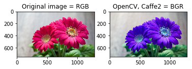
Note : OpenCV actually stores color in the BGR format.

Why? We use BRG order on computers due to how unsigned 32-bit integers are stored in memory, it still ends up being stored as RGB. The integer representing a color e.g. 0x00BBGGRR will be stored as 0xRRGGBB00.

CMYK Color Space

CMY Model

CMY means Cyan, Magenta and Yellow.

Secondary Colors of light or primary colors of pigments
Model for printers (color pigments on paper)

CMYK Model

Sometimes, a CMYK model (K stands for Black) is used in color printing to produce darker black.

^ CMY and CMYK is not really related to OpenCV. Just for your information.

HSV Color Space

HSV (Hue, Saturation & Value/Brightness) is a color space that attempts to represent colors the way human perceive it. It stores color information in a cyclindrical representation of RGB color points.

HSV Color Model

Hue - Color Value (0-179)
Saturation - Vibrancy of Color (0-255)
Value - Brightness or Intensity (0-255)

HSV is useful in computer vision for color segmentation. In RGB, filtering specific colors isn’t easy. However, HSV makes it much easier to set color ranges to filter specific colors as we perceive them.

Color Filtering

The Hue (Hue color range, goes from 0 to 180. NOT 360) and is mapped differently than standard in OpenCV.

Color Range Filters:

Red - 165 to 15
Green - 45 to 75
Blue - 90 to 120

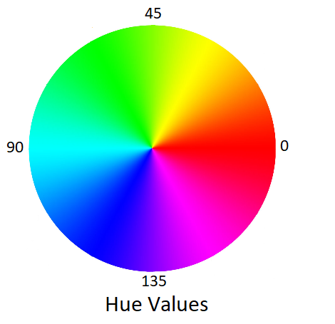
Why is the range of Hue 0-180° in OpenCV?

Now you understand why I said Hue is 0-179 in HSV space. 180 = 0.

Color Space

How Color Space affect the color levels

Note OpenCV’s RGB is not RGB but BGR.

import cv2

# Load image
image = cv2.imread('./images/Z.jpg')

# Look for individual color BGR values for the first pixel (0,0)
B, G, R = image[0,0]

print(B,G,R)
# ^ Return values of B, G, R respectively

print(image.shape)
# ^ Return values of Height, Width, and the last value '3' means we are using RGB values

Now lets convert it to grayscale.

# Convert to grayscale
gray_image = cv2.cvtColor(image, cv2.COLOR_BGR2GRAY)

print(gray_image.shape)
# ^ Return 2 values because it is on 2 dimensions now

print(gray_image[0,0])
# ^ Return a value of the gray level

Convert Image into HSV color space

import cv2
#H: 0 - 180, S: 0 - 255, V: 0 - 255

image = cv2.imread('./images/Z.jpg')
hsv_image = cv2.cvtColor(image, cv2.COLOR_BGR2HSV)

cv2.imshow('HSV image', hsv_image)
cv2.imshow('Hue channel', hsv_image[:,:,0]) 
cv2.imshow('Satuartion channel', hsv_image[:, :, 1])
cv2.imshow('Value channel', hsv_image[:, :, 2])
# ^ [:,:] here meaning all height and width

cv2.waitKey()
cv2.destroyAllWindows()

The HSV image looks quite cool.

Individual Channels in an RGB Image

Amplifying

import cv2

image = cv2.imread('./images/Z.jpg')

# OpenCV's 'spilt' function splites the image into each color index
B, G, R = cv2.split(image)

print(B.shape)

cv2.imshow("Red", R)
cv2.imshow("Green", G)
cv2.imshow("Blue", B)
cv2.waitKey(0)
cv2.destroyAllWindows()

# ^ Press Any key to continue...

# Let's re-make the original image
merged = cv2.merge([B,G,R])
cv2.imshow("Merged", merged)

# Let's amplify the blue color
merged = cv2.merge([B+100,G,R])
cv2.imshow("Merged with Blue Amplified", merged)

cv2.waitKey(0)
cv2.destroyAllWindows()

Only One Color

import cv2
import numpy as np

image = cv2.imread('./images/Z.jpg')
B, G, R = cv2.split(image)

# Let's create a matrix of zeros
# with dimensions of the image h x w
zeros = np.zeros(image.shape[:2], dtype = "uint8")
# ^`np.zeros()` makes every elements in this array become 0.

cv2.imshow("Red", cv2.merge([zeros, zeros, R]))
cv2.imshow("Green", cv2.merge([zeros, G, zeros]))
cv2.imshow("Blue", cv2.merge([B, zeros, zeros]))

cv2.waitKey(0)
cv2.destroyAllWindows()

1
2
3

print(image.shape[:2])
#^ this means the height and width of image. 
#Same as print(image.shape[0], image.shape[1]) but put a one

Histogram

Histogram are a great way to visualize individual color components of Images

Import Matplotlib

To Create Histogram we need to import the matplotlib.

1	from matplotlib import pyplot as plt

Function cv2.calcHist()

We will use a function cv2.calcHist().

cv2.calcHist(images,channels,mask,histSize,ranges[, hist[, accumulate]] )

images - source image, given in square brackets

channels - [0] for grayscale, [0] or [1] or [2] for color image (blue, green or red channel)

mask - for finding particular region of image

histSize - [256] for full scale

ranges - Normally [0, 256]

1 2	image = cv2.imread('./images/Z.jpg') histogram = cv2.calcHist([image],[0], None, [256], [0, 256])

Plot it out

Now let’s plot it out.

# we plot a historgram, `ravel()` flatens our image array
plt.hist(image.ravel(), 256, [0, 256]); plt.show()

# Viewing Separate Color Channels
color = ('b', 'g', 'r')

# We now separate the colors and plot each in the Histogram
for i, col in enumerate(color):
  histogram2 = cv2.calcHist([image],[i], None, [256], [0, 256])
  plt.plot(histogram2, color = col)
  plt.xlim([0,256])
  
plt.show()

Full Code

import cv2
import numpy as np

from matplotlib import pyplot as plt

image = cv2.imread('./images/Z.jpg')
histogram = cv2.calcHist([image],[0], None, [256], [0, 256])

# we plot a historgram, `ravel()` flatens our image array
plt.hist(image.ravel(), 256, [0, 256]); plt.show()

# Viewing Separate Color Channels
color = ('b', 'g', 'r')

# We now separate the colors and plot each in the Histogram
for i, col in enumerate(color):
  histogram2 = cv2.calcHist([image],[i], None, [256], [0, 256])
  plt.plot(histogram2, color = col)
  plt.xlim([0,256])
  
plt.show()

Output :

Drawing

You can use OpenCV to draw images and shapes.

To Plot the Image, use plt.imshow(image).

Note plt.imshow(image) uses RGB instead of BGR.

You might want to use cv2.cvtcolor(img,cv2.COLOR_BGR2RGB) to change it back to RGB for ploting.

For photos, you can use plot for quicker access.

Drawing a Square

# Create a black color image
c_image = np.zeros((512,512,3), np.uint8)

# Create a black and white image
bw_image = np.zeros((512,512), np.uint8)

cv2.imshow("Black Rectangle (Color)", c_image)
cv2.imshow("Black Rectangle (B&W)", bw_image)

cv2.waitKey(0)
cv2.destroyAllWindows()

Drawing a Line

cv2.line(image,starting cordinates, ending cordinates, color, thickness)

image - your image to draw on

starting cordinates - (x,y)

ending cordinates - (x,y)

color - (Blue value, Green value, Red value)

thinkness - measured in pixel

# Create a black color image
image = np.zeros((512, 512, 3), np.uint8)

# Draw a diagonal blue line of thickness of 5 pixels
cv2.line(image, (0,0), (511,511), (255,127,0), 5)

cv2.imshow("Blue Line", image)
cv2.waitKey(0)
cv2.destroyAllWindows()

Drawing a Rectangle

cv2.rectangle(image,starting vertex, opposite vertex, color, thickness)

# Draw a Rectangle in
image = np.zeros((512, 512, 3), np.uint8)

cv2.rectangle(image, (100, 100), (300, 250), (127, 50, 127), 5)
cv2.imshow("Rectangle", image)
cv2.waitKey(0)
cv2.destroyAllWindows()

Drawing a Circle

cv2.circle(image, center, radius, color, fill)

image = np.zeros((512, 512, 3), np.uint8)

cv2.circle(image, (350, 350), 100, (15, 75, 50), -1)
cv2.imshow("Circle", image)
cv2.waitKey(0)
cv2.destroyAllWindows()

Drawing Polygons

image = np.zeros((512,512,3), np.uint8)

# Let's define four points
pts = np.array( [[10,50], [400,50], [90,200], [50,500]], np.int32)

# Let's reshape our points in form required by polylines
pts = pts.reshape((-1,1,2))

cv2.polylines(image, [pts], True, (0,0,255), 3)
cv2.imshow("Polygon", image)
cv2.waitKey(0)
cv2.destroyAllWindows()

Adding Text

cv2.putText(image, text, starting point, font, font size, color, thickness)

image - your image to draw on

text - The text you want to display

starting point - (x,y) from botton left

font

cv2.FONT_HERSHEY_SIMPLEX or cv2.FONT_HERSHEY_PLAIN`

cv2.FONT_HERSHEY_DUPLEX or cv2.FONT_HERSHEY_COMPLEX`

cv2.FONT_HERSHEY_TRIPLEX or cv2.FONT_HERSHEY_COMPLEX_SMALL`

cv2.FONT_HERSHEY_SCRIPT_SIMPLEX

cv2.FONT_HERSHEY_SCRIPT_COMPLEX

font size - measured in pixel

color - (Blue value, Green value, Red value)

thinkness - measured in pixel

image = np.zeros((512,512,3), np.uint8)

cv2.putText(image, 'ZZZZZZZZZZ', (75,290), cv2.FONT_HERSHEY_COMPLEX, 2, (100,170,0), 3)

cv2.imshow("Text Showcase", image)
cv2.waitKey(0)
cv2.destroyAllWindows()