
Java - Time Complexity and Sorting
Big O Notation
- The Big O notation estimates the execution time of an algorithm in relation to the input size.
Best, Worst, and Average Cases
Best-case is not representative.
Worst-case is not representative, but worst-case analysis is very useful. You can show that the algorithm will never be slower than the worst-case.
Average-case analysis is ideal, but difficult to perform, because it is hard to determine the relative probabilities and distributions of various input instances for many problems.
Determining Big O Notation
Ignoring Multiplicative Constants
Algorithm analysis is focused on growth rate. The multiplicative constants have no impact on growth rates.
O(n/2) = O(100n) = O(n)
They are all the same so can be represented as O(n).
Ignoring Non-Dominating Terms
Algorithm analysis is for large input size. If the input size is small, there is no significance to estimate an algorithm’s efficiency.
O(n-1) = O(n)
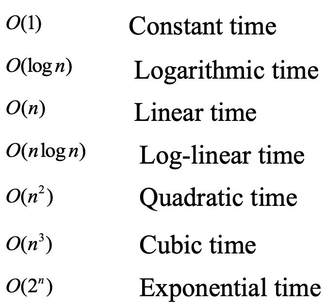
Common Big O Notation
Constant Time
O(1)
- If the time is not related to the input size, the algorithm is said to take constant time with the notation O(1).
Quadratic Time
O(n^2)
- If you double the input size, the time for the algorithm is quadrupled.
- Algorithms with a nested loop are often quadratic.
Logarithmic Time
O(log n)
- The base of the log is 2, but the base does not affect a logarithmic growth rate, so it can be omitted.
- The logarithmic algorithm grows slowly as the problem size increases.
- If you square the input size, you only double the time for the algorithm.
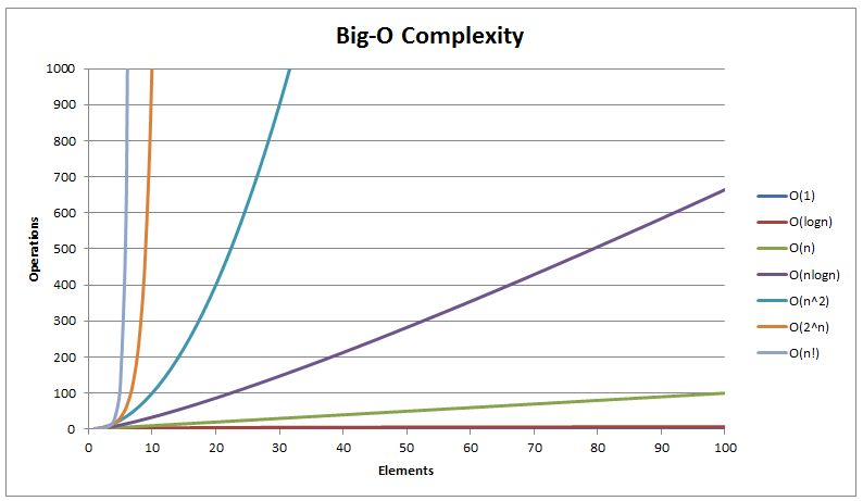
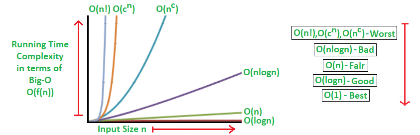
Comparing Common Growth Functions
O(1) < O(log n) < O(n) < O(n log n) < O(n^2) < O(n^3) < O(2^n)
Sorting
Why study sorting?
- sorting algorithms illustrate many creative approaches to problem solving and these approaches can be applied to solve other problems.
- sorting algorithms are good for practicing fundamental programming techniques using selection statements, loops, methods, and arrays.
- sorting algorithms are excellent examples to demonstrate algorithm performance.
Visualgo to Visualize Sorting Algorithms
Insertion Sort and Bubble Sort
Both Done by Swaping
Insertion Sort
- Done by swaping adjacently
- put the number at i into correct order by “inserting”

Best Case of Bubble Sort: O(n)
Worse Case of Bubble Sort: O(n^2)
Average Case of Bubble Sort: O(n^2)
1 | /*Function to sort array using insertion sort*/ |
Best Case of Insertion Sort: O(n)
Worse Case of Insertion Sort: O(n^2)
Average Case of Insertion Sort: O(n^2)
Bubble Sort
- Done by swaping adjacently
- Each iteration check number at i and number at i+1
- swap them if the it is not in order
- Each iteration check number at i and number at i+1

Insertion Sort vs Bubble Sort
Merge Sort and Quick Sort
Both done by Divide and Conquer.
Merge Sort
Merge Sort is a Divide and Conquer Algorithm.
- Keep Dividing the Array into 2 parts until the array size become 1.
- After Dividing them to smallest size, merging start.
- Merging based on compasion of elements
Best Case of Merge Sort: O(n log n)
Worse Case of Merge Sort: O(n log n)
Average Case of Merge Sort: O(n log n)
1 |
|
Quick Sort
- Pivot divide array into 2 halfs
- A pivot can be chosen arbitrarily.
- A pivot divides a list into two sublists,
- the elements in the first list are smaller than the pivot
- the elements in the second list are larger than the pivot.
If two subpivot is not meeting the requirement (i.e. low is not < pivot, high is not > pivot), Swap them
When low subpivot and high subpivot is pointing to same number, from now on we need a new partition. We swap high subpivot with pivot when high subpivot is lower than pivot.
Quick Sort Partition Animation
https://stackoverflow.com/questions/6740183/quicksort-with-first-element-as-pivot-example
For example: make a first partition
5 2 9 3 8 4 0 1 6 7 (using first element 5 as pivot)
firstly, subpivot low is 2 while subpivot high is 7.
2 < 5 and 7 > 5 therefore both low and high subpivot point to next number (that is 9 and 6).
9 is not < 5 and 6 > 5, therefore low subpivot stops, high subpivot point to next number (that is 1).
1 is not > 5, In this moment the numbers in both subpivot swaps (1 and 9).
5 2 1 3 8 4 0 9 6 7
subpivot further moves. Both low and high subpivot is now point to next number (that is 3 and 0).
3 < 5 and 0 is not > 5, therefore high subpivot stops, low subpivot point to next number (that is 8).
8 is not < 5, In this moment the numbers in both subpivot swaps (8 and 0).
5 2 1 3 0 4 8 9 6 7
subpivot further moves. Both low and high subpivot is now point to next number (that is 4 and 4).
Since now the low subpivot and high subpivot is pointing to same number, from now on we need a new partition. We swap high subpivot with pivot when high subpivot is lower than pivot.
4 is not > 5, therefore high subpivot stops. the number of high subpivot and pivot are swapped.
Note the pivot is still pointing at 5.
4 2 1 3 0 5 8 9 6 7
Best Case of Quick Sort: O(n log n)
Worse Case of Quick Sort: O(n^2)
Average Case of Quick Sort: O(n)
1 |
|
Merge Sort vs Quick Sort
